05 · Joints and actuators


Part	1 · Simulation
Run type	CPU · Mac or Colab CPU
Prerequisites	01, 02
Learn first	Calculus for Machine Learning
Time	~45 min
Code	`experiments/05-joints-and-actuators/experiment.py`
Status	✅ done

Act on this lesson

Tick each step when you have done it. Saved in this browser only.

01 · Read The problem and the core idea; answer the questions before you read.
02 · Build it Type the steps yourself, then run uv run python experiments/05-joints-and-actuators/build.py
03 · Run the experiment Predict first, then run uv run python experiments/05-joints-and-actuators/experiment.py
04 · Break it Change the one parameter and watch it fail.
05 · Check yourself Quizzes and exercises at the end.

A <position> actuator is a PD controller living inside the physics step: its gain sets the sag, and the armature decides whether the step can integrate it.

The problem

The Menagerie SO-101 gives every joint the same servo: <position kp="998.22" kv="2.731" forcerange="-2.94 2.94"/> on a joint with armature="0.028", and a comment says these gains are not a one-to-one copy of the real servo’s (so101.xml). Why is kp almost 1000, what does armature do on a hobby servo, and what happens if you copy the gains but drop the armature? This lesson builds one gravity-loaded link, measures how kp sets sag and rise time, and finds where the same gains make the simulation diverge.

Before you read · 2 questions. Guess first; the lesson tells you why.

1. A <position> servo holds a link against gravity. You raise kp from 10 to 100. What happens to the sag and the rise time?

The sag drops to zero; the rise time stays the same.
Both fall ten times.
The sag falls about ten times, the rise time only by about $\sqrt{10}$ .

Why: Sag $\approx \tau_g/k_p$ and rise time $\propto 1/\sqrt{k_p}$ . In the kp sweep the sag goes 1.685° → 0.169° and the rise time 185.6 → 56.7 ms.

2. The SO-101 model adds armature="0.028" to every joint. In a real geared servo, what does armature stand for?

The friction in the gearbox.
The spinning motor rotor, which the gearbox makes feel much heavier at the joint (rotor inertia × gear ratio²).
The mass of the servo’s plastic case.

Why: Armature adds to the joint’s diagonal of the mass matrix; for a geared motor it is the reflected rotor inertia (In plain words, Math details). Numerically it lowers $\omega = \sqrt{k_p/I}$ .

Core idea

In plain words

A <position> actuator behaves like a spring plus a shock absorber pulling the joint toward the commanded angle. The spring’s stiffness is kp: the further from the target, the harder it pulls. The shock absorber’s strength is kv: the faster the joint moves, the more it brakes. Engineers call this a PD controller (Proportional to the error, plus a Derivative term on the speed).

A weight on a spring settles below its unloaded rest: a spring pushes only when stretched. A position servo under gravity does the same: it sags, by roughly the gravity torque divided by kp. A stiffer spring sags less and arrives sooner.

Stiffness has a price in simulation. A stiff spring on a light joint oscillates fast; when one timestep is long compared with that oscillation, each step overshoots and the simulation explodes. Armature is extra inertia added to the joint: in a real servo, the motor’s spinning rotor, which the gearbox makes feel much heavier at the joint. It slows the oscillation so the timestep can follow.

flowchart TD
    U["command u<br/>(target angle)"] --> A["position actuator<br/>kp·(u − q) − kv·q̇"]
    A --> L["clamp to forcerange"]
    L --> J["joint with inertia<br/>I = I_link + armature"]
    G["gravity torque<br/>τ_g · cos q"] --> J
    J --> S["integrator step h"]
    S -- "new q, q̇" --> A

The servo, as code

force = clip(kp * (u - q) - kv * qdot, *forcerange)   # spring toward u, damper on speed (PD), clamped

# Steady sag e under a gravity torque tau_g: solve kp * e == tau_g * cos(e)
sag_estimate = tau_g / kp                        # good when the sag is small

# How fast the joint oscillates, and whether the timestep h can follow it
omega = sqrt(kp / (I_link + armature))           # natural frequency (rad/s)
h_omega = h * omega                              # explicit integration needs about h_omega < 2
kv = 2 * zeta * sqrt(kp * m)                     # what dampratio=zeta sets; m = reflected inertia

Quantity	Formula
actuator force	$k_p(u - q) - k_v\,\dot q$ , clamped to `forcerange`
steady sag	$k_p\,e_{\text{ss}} = \tau_g \cos e_{\text{ss}}\ \ (\approx \tau_g/k_p)$
natural frequency	$\omega = \sqrt{k_p / I}$ , with $I = I_{\text{link}} + \text{armature}$
explicit stability limit (undamped)	$h\omega \lesssim 2$
`implicitfast` limit with damping	$h^2\omega^2 < 4 + 2hc$ , with $c = (k_v + \text{damping})/I$
`kv` from `dampratio`	$k_v = 2\zeta\sqrt{k_p\,m}$

$u$ is the commanded angle, $q$ the joint angle, $\dot q$ its speed; $k_p$ , $k_v$ the actuator gains; $\tau_g$ the gravity torque with the link horizontal; $e_{\text{ss}}$ the steady-state error (sag); $I$ the effective inertia, $I_{\text{link}}$ the link’s part; $h$ the timestep; $c$ the damping per unit inertia; $\zeta$ the damping ratio, $m$ the reflected inertia at qpos0.

Math details: sag, rise time and the two stability bounds

Sag. At rest $\dot q = 0$ and $k_p(0 - q) = \tau_g\cos q$ at $q = -e_{\text{ss}}$ ; for small $e_{\text{ss}}$ , $e_{\text{ss}} \approx \tau_g/k_p$ . Without an integral term (one that grows while the error persists) the error never reaches zero.

Rise time. Linearized around the target, the joint is a mass on a spring with time scale $1/\omega = \sqrt{I/k_p}$ ; at fixed damping ratio every timing scales with it, hence $\propto 1/\sqrt{k_p}$ .

Explicit limit. Euler, implicit and implicitfast integrate the position term explicitly; the docs give the limit $h \lesssim 2/\omega_{\max}$ and note that only discrete is implicit in position (Computation · Integrators), the $h\omega < 2$ of lessons 02 and 03.

With implicit damping. implicitfast evaluates the damping at the new velocity: $v' = v + h(-\omega^2 q - c\,v')$ , $q' = q + h v'$ . The step matrix has determinant $1/(1 + hc)$ and trace $(2 + hc - h^2\omega^2)/(1 + hc)$ ; a 2×2 linear map is stable when $|\text{trace}| < 1 + \det$ , i.e. $h^2\omega^2 < 4 + 2hc$ . Damping integrated explicitly (Euler’s treatment of kv) gives $h^2\omega^2 < 4 - 2hc$ : it lowers the limit. Build it, Step 4 computes both numerically.

Armature. Armature adds to the joint’s diagonal of the mass matrix $M$ ; for a geared motor it is the reflected rotor inertia, rotor inertia × gear ratio² (XML reference · joint). A larger $I$ lowers $\omega$ .

Go deeper: Calculus for Machine Learning (AIEFS: linearization around the setpoint); MuJoCo Modeling · Actuators.

Joints

`joint type`	dof	Typical use
`hinge`	1 rotation about `axis`	every SO-101 joint
`slide`	1 translation along `axis`	linear stages, prismatic grippers
`ball`	3 rotations	rarely in arms
`free`	6	floating bodies, robot bases

Joint attribute	Effect	Source note
`range`	position limit (a soft constraint, like contact)	enabled by `limited` or `autolimits`
`damping`	$\tau = -\text{damping}\cdot\dot q$	`Euler` treats it implicitly
`armature`	extra inertia on the joint’s diagonal of $M$	rotor inertia × gear ratio²
`frictionloss`	dry friction that does not scale with a normal force	a constraint, not a force law

Sources: XML reference · joint, Computation · Friction loss.

Actuators

Every actuator is general: force $= \text{gain}\cdot\text{ctrl} + \text{bias}$ , clamped to forcerange, mapped to the joint through gear (Build it, Step 1). The shortcuts set gain and bias (XML reference · actuator, Modeling · Actuators):

Shortcut	Force	Notes
`motor`	$u$	torque command; the policy is the controller
`position`	$k_p(u - q) - k_v\,\dot q$	built-in PD; `kp` default 1, `kv` default 0, or `dampratio`
`velocity`	$k_v(u - \dot q)$	the docs recommend `implicitfast`/`implicit` with it

Build it

You will now write MuJoCo’s actuator force law and the Experiment’s servo-driven link in about 40 lines of NumPy, reproduce the kp sweep, and predict every cell of Break it from a 2 × 2 matrix. Type the steps into your own file and run it after each step. The finished functions are in physai/sim.py; uv run python experiments/05-joints-and-actuators/build.py runs all four steps with the checks (output in build_output.txt).

Step 1 · One force law for every actuator

Every actuator is affine: force = gainprm[0] · ctrl + biasprm[0] + biasprm[1] · length + biasprm[2] · velocity, then clamped. The shortcuts only fill these numbers: position sets gain $k_p$ and bias $(0, -k_p, -k_v)$ , velocity gain $k_v$ and bias $(0, 0, -k_v)$ , motor gain 1.

def actuator_force(ctrl, length, velocity, gainprm, biasprm, forcerange=None):
    """MuJoCo's affine actuator: gain * ctrl + bias(length, velocity), then clamped to forcerange."""
    force = gainprm[0] * ctrl + biasprm[0] + biasprm[1] * length + biasprm[2] * velocity
    return force if forcerange is None else np.clip(force, *forcerange)

For a joint actuator the length is the joint angle and the torque is gear × force. Three hinges, one actuator each:

== Step 1. Actuator force laws vs MuJoCo (100 random states and controls) ==
motor, gear 3                        gainprm[0]   1.0 · biasprm[:3] [0. 0. 0.] · max error 0.0e+00 N m
position kp 40 kv 2, forcerange ±5   gainprm[0]  40.0 · biasprm[:3] [  0. -40.  -2.] · max error 3.6e-15 N m
velocity kv 0.7                      gainprm[0]   0.7 · biasprm[:3] [ 0.   0.  -0.7] · max error 0.0e+00 N m

Step 2 · The Experiment’s link

Three numbers set the servo’s behaviour, each computable by hand: the inertia about the hinge (lesson 01’s capsule solid_inertia plus the parallel-axis term $m (L/2)^2$ ), gravity $-\tau_g\cos q$ , and $k_v$ from dampratio through the inertia, link plus armature:

def kv_from_dampratio(kp, dampratio, inertia):
    """Damping gain that gives a position servo this damping ratio on this inertia: 2 zeta sqrt(kp I)."""
    return 2 * dampratio * np.sqrt(kp * inertia)

== Step 2. The Experiment's link: inertia, gravity torque, kv from dampratio ==
link inertia about the hinge 0.00414684 kg m^2 · M_00 - armature 0.00414684
gravity torque at q = 0.3: -tau_g cos q = -0.281156 N m · -qfrc_bias -0.281156 N m
   kp  kv ours  kv MuJoCo
    1    0.359      0.359
   10    1.134      1.134
  100    3.586      3.586
 1000   11.340     11.340

The Experiment’s tables use the thin-rod $mL^2/3$ = 0.0040 kg·m²; the capsule’s rounded ends add 0.00015, so Step 4’s $h\omega$ differs from Break it A in the second decimal.

Step 3 · The servo loop

implicitfast treats every velocity-dependent force implicitly, here the actuator’s $k_v$ , so the step is lesson 01’s semi_implicit_euler with c_implicit = $k_v / I$ :

accel = lambda q, v: (actuator_force(0.0, q, v, [kp], [0, -kp, -kv]) - tau_g * np.cos(q)) / I
q, v = semi_implicit_euler(q, v, accel, h, c_implicit=kv / I)     # one implicitfast step

The sag solves $k_p e = \tau_g\cos e$ (Newton’s method):

def servo_sag(kp, tau_g):
    """Steady error e of a PD servo holding a link against gravity: kp e = tau_g cos e (Newton's method)."""
    e = tau_g / kp
    for _ in range(50):
        e -= (kp * e - tau_g * np.cos(e)) / (kp + tau_g * np.sin(e))
    return e

== Step 3. Our servo loop vs mj_step (implicitfast), step -0.5 rad -> 0, 3 s ==
   kp  max |q_ours - qpos|  sag (deg)  servo_sag (deg)  rise 10-90 % (ms)
    1              5.6e-17     16.193           16.193              533.0
    3              1.4e-17      5.594            5.594              335.6
   10              2.8e-17      1.685            1.685              185.6
   30              2.8e-17      0.562            0.562              106.1
  100              1.4e-17      0.169            0.169               56.7
  300              5.6e-17      0.056            0.056               31.6
 1000              2.8e-17      0.017            0.017               16.5

The Experiment’s sweep, row for row, and a trajectory within 6e-17 rad of mj_step.

Step 4 · Predict Break it

step_growth passes keyword arguments to the step, so it compares both integrators on the linearized servo, $a = -(k_p/I)\,q - ((k_v + \text{damping})/I)\,v$ . Euler treats only the joint damping implicitly; implicitfast treats $k_v$ too:

g_euler = step_growth(semi_implicit_euler, h, kp / I, (kv + damping) / I, c_implicit=damping / I)
g_fast = step_growth(semi_implicit_euler, h, kp / I, (kv + damping) / I, c_implicit=(kv + damping) / I)

== Step 4. Growth per step: kv explicit (Euler) or implicit (implicitfast) vs MuJoCo ==
      kp armature   h*w  Euler growth  MuJoCo Euler  implicitfast growth  MuJoCo implicitfast
     998    0.028  0.88         0.725        stable                0.812               stable
     998    0.010  1.33         0.343        stable                0.678               stable
     998    0.005  1.65         1.650      diverged                0.595               stable
     998    0.002  2.01         2.838      diverged                0.519               stable
     998    0.000  2.45         4.143      diverged                0.446               stable
    3000    0.028  1.53         0.725        stable                0.812               stable
   10000    0.028  2.79         5.491      diverged                3.262             diverged
   30000    0.028  4.83        19.786      diverged               13.661             diverged

Growth above 1 marks exactly the cells where MuJoCo diverges, in both integrators, although the linear test leaves out frictionloss. It is Math details’ bound, computed: explicit damping lowers the limit (Euler fails at $h\omega$ = 1.65), implicit damping raises it (implicitfast holds at 2.45 without armature, but not at kp 10000, $h\omega$ = 2.79, where $hc$ is small).

What you keep

physai.sim now has actuator_force, kv_from_dampratio and servo_sag, and semi_implicit_euler with c_implicit is an implicitfast step. Lesson 12 writes the full joint controller (PID, gravity feedforward) next to it. tests/test_05_joints_and_actuators.py pins them to MuJoCo; run uv run pytest tests/test_05_joints_and_actuators.py after you change anything.

Use it

Declare the actuator, let mj_step apply it, read the compiled numbers back:

<position joint="j" kp="998.22" kv="2.731" forcerange="-2.94 2.94"/>   # or dampratio="1" instead of kv

d.ctrl[a] = target                                  # in ctrlrange; for <position>, an angle
mujoco.mj_step(m, d)
d.actuator_force[a]                                 # force after the clamp (Step 1)
d.qfrc_actuator                                     # joint torques: gear x force
m.actuator_gainprm[a, 0], m.actuator_biasprm[a, :3] # kp and (0, -kp, -kv)

Traps:

<general> ignores biasprm unless you also set biastype="affine" (the default is none); <position> sets it for you.
Two clamps. ctrlrange limits the command (for <position>, an angle), forcerange the force.
dampratio is resolved at compile time from the inertia at qpos0 (Step 2); change the armature or a mass at runtime and $k_v$ keeps its old value.

Check after building · 2 questions.

1. In Build it, Step 1, <position kp="40" kv="2"/> compiles to gainprm[0] = 40 and biasprm[:3] = (0, −40, −2). Which force does actuator_force compute from these numbers?

$40\,u - 2\,\dot q$ , with no term in $q$ .
$40\,(u - q)$ , because the damping is applied by the integrator.
$40\,u - 40\,q - 2\,\dot q = k_p(u - q) - k_v\dot q$ , then clamped to forcerange.

Why: Force = gain · ctrl + bias₀ + bias₁ · length + bias₂ · velocity; for a joint actuator the length is the joint angle (times gear). The hand-written law matches actuator_force to 3.6e-15 N m.

2. In Build it, Step 4, the SO-101 servo with armature 0.005 has growth 1.650 under Euler (MuJoCo diverges) but 0.595 under implicitfast (stable). What differs between the two steps?

implicitfast also treats the actuator’s $k_v$ implicitly (c_implicit = $(k_v + \text{damping})/I$ ), which raises the limit to $h^2\omega^2 < 4 + 2hc$ ; Euler treats only the joint damping implicitly.
implicitfast uses a smaller timestep internally.
implicitfast integrates the position term implicitly as well.

Why: Only discrete is implicit in position. With $k_v$ explicit the damping lowers the bound ( $h^2\omega^2 < 4 - 2hc$ ), so Euler already fails at $h\omega$ = 1.65; the growth column marks exactly the cells where MuJoCo diverges.

Experiment

A 20 cm, 0.3 kg capsule on a hinge, horizontal at $q = 0$ : $\tau_g$ = 0.2943 N·m, $I_{\text{link}}$ = 0.0040 kg·m² (thin rod), dt = 5 ms (the SO-101 timestep), implicitfast.

<option timestep="0.005" integrator="implicitfast"/>
<body name="link">
  <joint name="j" type="hinge" axis="0 -1 0" armature="0.028"/>
  <geom type="capsule" fromto="0 0 0 0.2 0 0" size="0.01" mass="0.3"/>
</body>
<actuator><position joint="j" kp="{kp}" dampratio="1"/></actuator>

Start at $q = -0.5$ rad, command $u = 0$ , run 3 s. Sag = mean error over the last 0.5 s; rise = time from 10 % to 90 % of the way.

Predict. kp × 10: what happens to sag, and to rise time?

Run. experiment.py, MuJoCo 3.17.0, NumPy 2.5.4, Apple M5, deterministic; output in output.txt.

kp (N·m/rad)	kv from dampratio 1	sag (°)	$\tau_g/k_p$ (°)	exact (°)	rise 10–90 % (ms)
1	0.359	16.193	16.862	16.193	533.0
3	0.621	5.594	5.621	5.594	335.6
10	1.134	1.685	1.686	1.685	185.6
30	1.964	0.562	0.562	0.562	106.1
100	3.586	0.169	0.169	0.169	56.7
300	6.211	0.056	0.056	0.056	31.6
1000	11.340	0.017	0.017	0.017	16.5

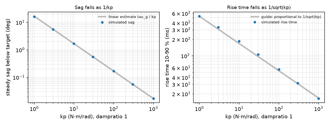
Two log-log plots against kp from 1 to 1000. Left: steady sag falls from 16.193° to 0.017° and lies on the tau_g/kp line except at kp 1. Right: rise time falls from 533.0 ms to 16.5 ms, close to a 1/sqrt(kp) guide line.

Observe. The sag equals the static balance $k_p e = \tau_g\cos e$ to three decimals in every row; the linear $\tau_g/k_p$ is off only when the sag is large (kp = 1). A position servo with no integral term always sags under gravity: 0.017° at kp 1000, 16.193° at kp 1. Rise time falls as $1/\sqrt{k_p}$ (kp 10 → 100: 185.6 → 56.7 ms). Removing the sag without huge gains is what gravity feedforward does in lesson 12.

Break it

A · keep the SO-101 servo, drop the armature. kp 998.22, kv 2.731, joint damping 0.6, frictionloss 0.052, dt = 5 ms; sweep armature:

armature	$I$ (kg·m²)	$h\omega$	Euler	implicitfast	discrete
0.028	0.0320	0.88	stable	stable	stable
0.010	0.0140	1.34	stable	stable	stable
0.005	0.0090	1.67	diverged	stable	stable
0.002	0.0060	2.04	diverged	stable	stable
0.001	0.0050	2.23	diverged	stable	stable
0	0.0040	2.50	diverged	stable	stable

Euler fails first, already at $h\omega$ = 1.67: it treats joint damping implicitly but the actuator’s kv explicitly, which is why the docs recommend implicitfast or implicit whenever kv is used (actuator/position/kv). With the Menagerie forcerange ±2.94 N·m added, Euler no longer explodes; it chatters (a fast, small back-and-forth around the target): peak-to-peak 0.629° at armature 0.001 and 0.798° at 0, a failure that looks like servo noise rather than numerics.

B · raise kp (implicitfast, armature 0.028): stable at kp 3000 ( $h\omega$ = 1.53), diverged at kp 10000 ( $h\omega$ = 2.80) and 30000 ( $h\omega$ = 4.84); discrete stayed stable at all four. implicitfast treats damping implicitly but kp explicitly, which gives the bound $h^2\omega^2 < 4 + 2hc$ with $c = (k_v + \text{damping})/I$ (Math details); the docs’ $h\omega \lesssim 2$ is the undamped case. With armature 0.028, $hc$ is small and the limit sits just above 2. In A, removing the armature made $I$ tiny and $hc$ large, so implicitfast survived $h\omega$ = 2.50 while Euler, with kv explicit, failed at 1.67. Build it, Step 4 predicts every cell of A and B this way.

On the real robot

The script reads the compiled SO-101 model (Menagerie · robotstudio_so101), home pose qpos0, dt = 5 ms:

joint	kp	kv	forcerange (N·m)	armature	$M_{ii}$ (kg·m²)	link part	$h\omega$	$h\omega$ without armature
shoulder_pan	998.22	2.731	±2.94	0.028	0.04446	0.01646	0.75	1.23
shoulder_lift	998.22	2.731	±2.94	0.028	0.04542	0.01742	0.74	1.20
elbow_flex	998.22	2.731	±2.94	0.028	0.03734	0.00934	0.82	1.63
wrist_flex	998.22	2.731	±2.94	0.028	0.02913	0.00113	0.93	4.71
wrist_roll	998.22	2.731	±2.94	0.028	0.02808	0.00008	0.94	17.62
gripper	998.22	2.731	±2.94	0.028	0.02802	0.00002	0.94	39.33

For the wrist and gripper the armature is almost the whole effective inertia; without it those joints would sit far past $h\omega \approx 2$ . Copying kp and kv without the armature into an Euler model reproduces Break it A. Whether the SO-101’s own implicitfast survives without armature was not tested; its large implicit kv raises the limit, so assume nothing.

Real hardware facts, from the LeRobot SO-101 guide: the follower uses six STS3215 servos with 1/345 gearing; the leader mixes 1/191, 1/345 and 1/147 so it can be moved by hand. The servos share one bus, each with a unique ID (shoulder pan 1 … gripper 6) stored in its EEPROM (non-volatile memory). The Menagerie comment states that its kp, kv and forcerange assume a servo proportional gain of 16 and are not a one-to-one mapping of LeRobot’s gains.

Procedure: command a 0.5 rad step on the real elbow, log the joint position through LeRobot, and compare rise time and sag with the simulated joint under the same load. Not yet measured on the real arm.

Check yourself

Quick check · 2 questions. Click an answer.

1. You copy the SO-101 servo gains (kp 998.22, kv 2.731) into a model at dt = 5 ms but drop the armature. What does Euler do?

It diverges already at armature 0.005 ( $h\omega$ = 1.67), because it integrates the actuator’s kv explicitly.
Nothing changes, because armature only models the rotor for display.
It stays stable down to $h\omega$ = 2, exactly as the undamped limit says.

Why: Break it A, Euler diverges from 0.005 on while implicitfast and discrete stay stable; with explicit damping the bound becomes $h^2\omega^2 < 4 - 2hc$ , below 2.

2. Why does the armature matter most for the SO-101’s wrist roll and gripper joints?

Those joints carry the largest gravity torque.
Their links are so light that the armature is almost their whole effective inertia; without it $h\omega$ would be 17.62 and 39.33.
They have the narrowest joint ranges, and armature acts as a soft limit.

Why: In the On the real robot table the link part is 0.00008 and 0.00002 kg·m² against an armature of 0.028; with it every joint stays below $h\omega$ = 1.

Easy. Replace <position> by <motor> and send ctrl = 0. What does the link do? What ctrl holds it horizontal?
Medium. Add gear="2" to the position actuator, keep kp = 100. Does the sag change? Explain with the gear’s effect on length and force.
Hard. For Break it A, find the largest armature at which Euler diverges with kv = 0 (keep joint damping 0.6). Compare with the $h\omega$ = 2 prediction.

Answers

It falls under gravity (zero torque). Holding it needs $u = \tau_g$ = 0.2943 N·m at $q = 0$ .
gear scales both the actuator length and the force mapping, so the joint stiffness becomes gear² × kp: expect about a quarter of the sag. Measure it.
Undamped: $h\omega = 2$ , i.e. $I = k_p (h/2)^2$ . The implicit joint damping widens the bound to $h^2\omega^2 < 4 + 2hc$ , so divergence starts at a smaller armature; Build it’s step_growth with kv = 0 finds it before you run the sweep.

Takeaways and sources

<position> = PD with gains kp, kv; sag under gravity is $\tau_g\cos e/k_p$ (16.193° at kp 1, 0.017° at kp 1000), rise time ∝ $1/\sqrt{k_p}$ .
Armature lowers $\omega = \sqrt{k_p/I}$ . The SO-101’s 0.028 is most of the wrist and gripper inertia and keeps $h\omega$ below 1 at 5 ms.
Euler breaks first (explicit kv), implicitfast once $h^2\omega^2 > 4 + 2hc$ (≈ 2 when damping is small), discrete held in every tested case; step_growth predicts each cell.

Next: lesson 06 · Rotations. Control on top of these actuators: lesson 12.

Sources

MuJoCo XML reference · joint, actuator (motor, position, velocity, general).
MuJoCo Modeling · Actuators; Computation · Integrators.
Menagerie · robotstudio_so101/so101.xml (class sts3215).
LeRobot SO-101 guide.
Our numbers: output.txt, build_output.txt.