39 · Domain randomization


Part	9 · Sim to real
Run type	CPU · Mac or Colab CPU
Prerequisites	33, 38
Learn first	Sim-to-Real Transfer · Bias-Variance Tradeoff
Time	~60 min
Code	`experiments/39-domain-randomization/experiment.py`
Status	✅ done

Act on this lesson

Tick each step when you have done it. Saved in this browser only.

01 · Read The problem and the core idea; answer the questions before you read.
02 · Build it Type the steps yourself, then run uv run python experiments/39-domain-randomization/build.py
03 · Run the experiment Predict first, then run uv run python experiments/39-domain-randomization/experiment.py
04 · Break it Change the one parameter and watch it fail.
05 · Check yourself Quizzes and exercises at the end.

If you cannot know the real parameters exactly, train on a range that contains them; make the range too narrow and the policy is brittle, too wide and it is timid.

The problem

System identification (lesson 38) narrows the gap between simulator and robot but never closes it: some parameters stay uncertain, and some change from day to day (payload, wear, temperature, a different floor). A controller or policy optimized on one nominal simulator exploits exactly the numbers it was given. Unitree’s open training code for its legged robots therefore draws a new ground friction coefficient for every simulated robot, randomize_friction = True, friction_range = [0.5, 1.25], and pushes the robots at random every 15 s (legged_robot_config.py); the Go2 configuration inherits these settings unchanged (go2_config.py). How wide should such a range be, and what does width cost?

Before you read · 2 questions. Guess first; the lesson tells you why.

1. A driver trains only on one simulator with exactly known grip and reaction delay. What happens in a real car that differs a little?

Nothing; small differences average out.
The driver misjudges corners, because the style exploits the exact numbers of that one simulator.
The driver becomes too cautious.

Why: Tuned on the nominal plant only, the controller is best there (0.165°) and worst on the real plants (5/32): it chose Kp = 117 with little damping, relying on a 5 ms delay.

2. If randomizing helps, why not make the training range as wide as possible?

A very wide range makes the policy cautious, worse on the plant you know and eventually on the real one too.
Wide ranges make simulation unstable.
Wide ranges need a GPU.

Why: Break it: at w = 2 the controller is soft (Kp 19.59), 2.201° nominal and 13/32 on the real plants, worse than the narrowest range (24/32 at w = 0.1).

Core idea

In plain words

Train a driver on one simulator only and they learn its exact quirks: where to brake, how much grip there is, how quickly the car reacts. Put them in a real car that differs a little and they misjudge every corner. Train them instead on many slightly different simulators, each with its own grip, weight and reaction delay, and they learn a driving style that works across the whole family. If the real car belongs to that family, it is, in Tobin et al.’s words, “just another variation”. This is domain randomization (DR).

The price: a driver who must handle everything from ice to dry asphalt drives more cautiously than one who only knows dry asphalt. A range that is too narrow gives a brittle policy; one that is too wide gives a timid one. It is the same trade-off as regularization in machine learning: a little generalizes better, too much underfits.

flowchart TD
    W["choose width w"] --> S["draw a simulator:<br/>mass, damping,<br/>friction, delay"]
    S --> R["run an episode,<br/>score the tracking error"]
    R --> O["optimizer (CEM)<br/>updates the controller"]
    O --> S
    O --> P["tuned controller"]
    P --> T["test on held-out<br/>'real' plants"]

Domain randomization, as code

The only change from ordinary training is where the score comes from: an average over randomly drawn simulators instead of one fixed simulator. In this lesson the optimizer is the cross-entropy method (CEM), a simple derivative-free search: sample candidate controllers, keep the best ones, move the sampling distribution toward them, repeat.

def expected_return(gains, w, n=10):
    plants = [sample_plant(w) for _ in range(n)]       # n random simulators of width w
    return mean(J(gains, p) for p in plants)           # J: return of one episode (here -RMS tracking error)

mu, sd = initial_mean, initial_spread                  # search distribution over (Kp, Kd, kg)
for it in range(12):                                   # CEM iterations
    cands = [normal(mu, sd) for _ in range(24)]        # candidate controllers
    elite = best(cands, key=lambda g: expected_return(g, w))
    mu, sd = mean(elite), std(elite)                   # move the search toward the best ones

What	Formula
Nominal training	$\pi^*_0 = \arg\max_\pi\ J(\pi;\xi_0)$
Domain randomization	$\pi^*_w = \arg\max_\pi\ \mathbb{E}_{\xi \sim p_w}\big[J(\pi;\xi)\big]$
Width in this lesson	scales $\in [2^{-w}, 2^{w}]$ (log-uniform), delay $\in [5, 5+40w]$ ms

$\pi$ is the policy (here the gains $K_p$ , $K_d$ , $k_g$ ), $\xi$ a vector of simulator parameters (mass, damping, friction, delay), $\xi_0$ its nominal value, $J(\pi;\xi)$ the return of the policy on the simulator with parameters $\xi$ , and $p_w$ the distribution of simulators with width $w$ .

Math details: why averaging over simulators helps, and when it cannot

Coverage. DR optimizes the average return over $p_w$ . If the real robot’s $\xi_{\text{real}}$ lies inside the support of $p_w$ (the set of simulators that can be drawn), the policy has been scored on simulators like it; if it lies outside, nothing in training checked that case.

Average vs worst case. As $w$ grows, the average is increasingly dominated by hard simulators (long delays, heavy links), so the optimum moves toward a cautious, worst-case controller. In the limit this approaches a minimax problem, $\max_\pi \min_\xi J(\pi;\xi)$ , which gives up nominal performance for guarantees.

The bias-variance analogy. Training on one $\xi_0$ is like fitting one data set exactly: low error there, high error on new data. A wider $p_w$ acts like regularization: higher error on the known plant (bias), lower sensitivity to the unknown one (variance) (see AIEFS: Bias-Variance Tradeoff).

Limits of a fixed controller. A controller with fixed gains must find one compromise for every $\xi$ . When the real variation is larger than what any single compromise can absorb, no width helps (Observe 4).

Prior work. Tobin et al. (arXiv 1703.06907) randomized rendering to train an object detector on simulated images only. Tan et al. (arXiv 1804.10332) randomized physical parameters, added perturbations and identified an actuator model and latency to move quadruped gaits from simulation to a real robot.

Go deeper: Sim-to-Real Transfer, Bias-Variance Tradeoff (AIEFS); de Boer et al., “A Tutorial on the Cross-Entropy Method” (2005).

The trade-off, and what to randomize

Width	Nominal sim	Real robot
0 (nominal only)	best	fails when $\xi_{\text{real}} \ne \xi_0$
just covers $\xi_{\text{real}}$	slightly worse	works
far wider	worse	worse again: the policy is tuned for the worst case

For an arm, randomize the parameters of lesson 38 (masses, damping, friction, armature, actuator gain) and the delay of lesson 37. Center the ranges on identified values and size them from the identification’s uncertainty.

Build it

You will now write the part of domain randomization that is not physics: the sampler, a coverage check, the averaged cost and the optimizer. The plant and its batched MuJoCo rollout stay the Experiment’s (Batch.rollout(gains, plants) runs one episode per row and returns its RMS tracking error). The finished functions are in physai/sim2real.py; uv run python experiments/39-domain-randomization/build.py runs the steps (output in build_output.txt).

Step 1 · The sampler

A log-uniform scale is $2^u$ with $u$ uniform in $[-w, w]$ : halving and doubling are equally likely, and the median is 1.

def dr_sample(rng, n, w, delay0=0.005, delay_per_w=0.040):
    """n random plants of width w: mass, damping and friction scales log-uniform in [2^-w, 2^w], delay uniform in
    [delay0, delay0 + delay_per_w * w] seconds. w = 0 returns n nominal plants and draws nothing from rng."""
    if w == 0:
        return dict(mass=np.ones(n), damping=np.ones(n), friction=np.ones(n), delay=np.full(n, delay0))
    s = lambda: 2.0 ** rng.uniform(-w, w, n)  # noqa: E731
    return dict(mass=s(), damping=s(), friction=s(), delay=rng.uniform(delay0, delay0 + delay_per_w * w, n))

== Step 1. The sampler at w = 0.5, 100,000 draws ==
mass      min 0.7071 max 1.4142 (2^-0.5 = 0.7071, 2^0.5 = 1.4142), median 0.9993, share above 1: 0.499
damping   min 0.7071 max 1.4142 (2^-0.5 = 0.7071, 2^0.5 = 1.4142), median 0.9983, share above 1: 0.497
friction  min 0.7071 max 1.4142 (2^-0.5 = 0.7071, 2^0.5 = 1.4142), median 0.9994, share above 1: 0.499
delay     min 5.00 ms, max 25.00 ms (formula 5-25 ms)
same draws as the Experiment's sampler (seed 7): True

The draws hit both formula bounds, half of them lie above 1, and with the same seed they equal the Experiment’s sampler draw for draw, which Step 4 relies on.

Step 2 · Coverage

Before training anything, ask which real plants a width can draw at all:

def inside_support(plants, w, delay0=0.005, delay_per_w=0.040):
    """For every plant and parameter: can the width-w training distribution draw this value?"""
    lo, hi, eps = 2.0 ** -w, 2.0 ** w, 1e-12
    out = {k: (plants[k] >= lo - eps) & (plants[k] <= hi + eps) for k in ("mass", "damping", "friction")}
    out["delay"] = (plants["delay"] >= delay0 - eps) & (plants["delay"] <= delay0 + delay_per_w * w + eps)
    return out

== Step 2. Coverage: real plants inside the training support (of 32) ==
    w  mass  damping  friction  delay  all four
 0.00     0        0         0      0         0
 0.10     0        6         2      0         0
 0.25     7       13         4      0         0
 0.50    32       28         6     25         5
 0.75    32       32        11     32        11
 1.00    32       32        20     32        20
 1.50    32       32        32     32        32
 2.00    32       32        32     32        32
largest real friction scale 2.48, largest real delay 28.8 ms

At $w$ = 0.5 only 5 of the 32 real plants are fully inside the training distribution; it takes $w$ = 1.5 to cover all of them, because of friction (up to ×2.48). Yet the Experiment’s best widths are 0.5–1.0 (27–28/32) and $w$ = 1.5 reaches only 23/32. Coverage is necessary for a guarantee, not sufficient for good transfer: the price of width is paid on every plant.

Step 3 · The averaged cost

Domain randomization replaces “cost on one simulator” by “mean cost over sampled simulators”. Scoring every candidate on the same sampled plants (common random numbers) keeps the comparison between candidates fair:

def expected_cost(rollout, gains, plants):
    """Mean cost of every controller (row of gains) over the same sampled plants (common random numbers).
    rollout(gain_rows, plant_rows) runs one episode per row and returns its cost."""
    n, k = len(gains), len(plants["delay"])
    tiled = {key: np.tile(v, n) for key, v in plants.items()}       # plants 0..k-1 for controller 0, then 1, ...
    return rollout(np.repeat(gains, k, axis=0), tiled).reshape(n, k).mean(axis=1)

== Step 3. The averaged cost: the Experiment's tuned controllers, re-scored ==
tuned at       Kp     Kd     kg  nominal deg  real mean deg  real < 2 deg
w = 0.00   117.36  0.914  0.679        0.165          3.525          5/32
w = 0.50    55.43  3.244  0.563        0.475          1.307         28/32

Re-scored with the gains printed in the Experiment’s table, both rows come back: 0.165° nominal and 5/32 for the nominal-only controller, 0.475° and 28/32 for $w$ = 0.5. The real mean of the first row, 3.525° against the table’s 3.526°, differs because the table’s gains are rounded to two decimals.

Step 4 · The cross-entropy method

CEM keeps a Gaussian over the parameters, samples candidates, keeps the cheapest quarter, and refits the Gaussian to them. The small sd_extra stops the search from collapsing onto one point before it has converged.

def cem(cost, mu, sd, lo, hi, rng, iters=12, pop=24, n_elite=6, sd_extra=0.02):
    """Cross-entropy method: draw pop candidates from N(mu, sd) clipped to [lo, hi], keep the n_elite cheapest,
    refit mu and sd to them (plus sd_extra, so the search never collapses), repeat. cost(x, rng) -> one per row."""
    for _ in range(iters):
        x = np.clip(mu + sd * rng.standard_normal((pop, len(mu))), lo, hi)
        elite = x[np.argsort(cost(x, rng))[:n_elite]]
        mu, sd = elite.mean(axis=0), elite.std(axis=0) + sd_extra
    return mu

== Step 4. CEM: a toy quadratic, then domain randomization at w = 0.5 ==
toy: minimum at [ 1.  -2.   0.5], CEM finds [0.980, -2.008, 0.503]
w = 0.5: Kp 55.43, Kd 3.244, kg 0.563; nominal 0.475 deg, real mean 1.307 deg, 28/32 below 2 deg

On the toy quadratic CEM lands within 0.02 of the minimum. On the plant it reproduces the Experiment’s $w$ = 0.5 row exactly (Kp 55.43, Kd 3.244, kg 0.563, 28/32), because the sampler consumes the random generator in the same order. The optimizer never sees a real plant; only the width of dr_sample connects it to them.

What you keep

physai.sim2real now has dr_sample, inside_support, expected_cost and cem. The capstone (lesson 44) reasons about the same coverage question for its camera calibration. tests/test_39_domain_randomization.py checks the distributions against SciPy: uv run pytest tests/test_39_domain_randomization.py.

Use it

There is no “randomize” call in MuJoCo: the knobs are model fields, writable between episodes without recompiling (m.body_mass, m.dof_damping, m.dof_frictionloss, m.geom_friction, …; delay with lesson 37’s delay attribute). The Experiment puts many copies of the joint into one model, so one mj_step advances a whole batch, and writes one entry per copy before each rollout. SciPy names the distribution:

from scipy import stats
scales = stats.loguniform(2 ** -w, 2 ** w).rvs(size=n, random_state=rng)   # same law as dr_sample's 2**u

== Use it. SciPy's log-uniform distribution; MuJoCo model fields as the knobs ==
Kolmogorov-Smirnov, our mass scales vs scipy.stats.loguniform(2^-0.5, 2^0.5): D = 0.0026, p = 0.50
randomized fields in the batched model: body_mass (32,), dof_damping (32,), dof_frictionloss (32,) (one entry per copy, written before each rollout)

Tool	Where the range lives	What is drawn
physai	`dr_sample(rng, n, w)`	mass, damping, friction scales and delay, every episode
`unitree_rl_gym`	`randomize_friction`, `friction_range = [0.5, 1.25]`, `added_mass_range` (config)	ground friction once per environment, from 64 buckets (`legged_robot.py`)
MuJoCo	model fields (`body_mass`, `dof_damping`, …)	whatever you write before `mj_step`

Traps:

Scale vs absolute. “Mass ×2” and “mass + 1” are different distributions: unitree_rl_gym’s added_mass_range adds a number to the base body’s mass (props[0].mass +=).
Per episode vs per environment. Drawing once per environment (as the friction buckets above) gives each robot one fixed floor for the whole run; drawing per episode, as here, changes it every episode.
Inertia goes with mass. Scaling body_mass without body_inertia makes a physically inconsistent link; the Experiment scales both.

Check after building · 2 questions.

1. Build it, Step 2 shows that at w = 0.5 only 5 of the 32 real plants lie fully inside the training distribution, yet the w = 0.5 controller succeeds on 28/32. What does that say?

The coverage check has a bug.
Full coverage is required for any success.
Coverage is needed for a guarantee, not for good transfer; at w = 1.5 all 32 are covered, but success drops to 23/32.

Why: Most of the gain comes from not trusting the exact delay; the price of width is paid on every plant.

2. Why does expected_cost score every candidate on the same sampled plants instead of drawing new plants per candidate?

To save random numbers.
So that the difference between two candidates comes from the candidates, not from one getting easier plants (common random numbers).
Because MuJoCo can simulate only one plant per model.

Why: With the same order of random draws, Build it, Step 4 reproduces the Experiment’s w = 0.5 row exactly (Kp 55.43, Kd 3.244, kg 0.563, 28/32).

Experiment

Setup. One arm joint with the STS3215 joint parameters of the Menagerie SO-101 (armature 0.028, damping 0.6, frictionloss 0.052, torque limit 2.94 N·m) carrying a 0.5 kg link with its center of mass at 15 cm (gravity torque up to 0.736 N·m). Torque control through a measurement delay. The “policy” is a three-parameter controller: PD tracking plus a gravity term $k_g\cos q_{\text{ref}}$ ,

$\tau = \operatorname{clip}\big(K_p(q_{\text{ref}} - \tilde q) + K_d(\dot q_{\text{ref}} - \dot{\tilde q}) + k_g\cos q_{\text{ref}},\ \pm 2.94\big),$

where $\tilde q$ is the delayed measurement. It is tuned with CEM (Build it, Step 4: 12 iterations × 24 candidates × 10 sampled plants each) to minimize RMS tracking error of a 3 s reference, $0.5\sin(2\pi\,0.4t) + 0.25\sin(2\pi\,1.1t+1)$ rad, at a 2 ms step. With width $w$ , every training episode draws mass, damping and friction-loss scales log-uniformly in $[2^{-w}, 2^{w}]$ and the delay uniformly in $[5, 5+40w]$ ms (nominal: scales 1, delay 5 ms).

Test. The nominal plant, and 32 held-out “real” plants never seen in training (invented for the test): mass ×1.10–1.39, damping ×0.80–1.56, friction ×1.02–2.48, delay 15.5–28.8 ms. Success: RMS error below 2°. Many copies of the joint live in one MuJoCo model so that one mj_step advances a whole batch.

Full script: experiments/39-domain-randomization/experiment.py. MuJoCo 3.17.0, NumPy 2.5.4, Python 3.14, Apple Silicon Mac (Apple M5), deterministic (fixed seeds), well under a minute of CPU. Predict: which width is best on the real plants, and what happens to nominal error as $w$ grows?

$w$	delay range [ms]	scale range	$K_p$	$K_d$	$k_g$	nominal RMS [°]	real mean [°]	real worst [°]	real success
0	5	1.00	117.36	0.914	0.679	0.165	3.526	6.025	5/32
0.1	5–9	0.93–1.07	99.98	4.484	0.307	0.227	1.607	3.260	24/32
0.25	5–15	0.84–1.19	74.77	4.276	0.523	0.252	1.490	3.368	23/32
0.5	5–25	0.71–1.41	55.43	3.244	0.563	0.475	1.307	3.293	28/32
0.75	5–35	0.59–1.68	45.19	2.672	0.461	0.736	1.228	3.118	27/32
1.0	5–45	0.50–2.00	30.41	1.969	0.591	1.224	1.233	3.419	27/32

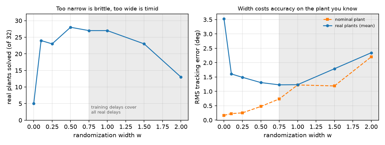
Observe.

Tuned on the nominal plant only, the controller is the best on that plant (0.165°) and the worst on the real ones (5/32). It chose $K_p$ = 117 with little damping, a loop that relies on knowing the delay is 5 ms; with 15.5–28.8 ms its error averages 3.526°.
Even a narrow range ( $w$ = 0.1, delay up to 9 ms) lifts real success to 24/32: most of the gain comes from not trusting the exact delay. The best results come from ranges whose delay reaches into the real 15.5–28.8 ms ( $w$ = 0.5 up to 25 ms; 0.75 and 1 all of it): 27–28/32, mean 1.228–1.307°, although only 5–20 of the 32 plants lie fully inside those ranges (Build it, Step 2). Each row is one CEM run with one seed; treat differences of a few plants as noise.
Nominal error grows steadily with width (0.165 → 1.224°) as $K_p$ falls (117 → 30): robustness is paid for in tracking on the plant you know.
No width solves all 32: the worst real plant stays above 3° in every row. Some real plants have friction ×2.48, outside even the $w$ = 1 range (up to ×2.00), and a fixed-gain controller has limits.

Break it

Make the range much wider than the real variation:

$w$	delay range [ms]	scale range	$K_p$	nominal RMS [°]	real mean [°]	real success
1.5	5–65	0.35–2.83	38.01	1.190	1.788	23/32
2.0	5–85	0.25–4.00	19.59	2.201	2.345	13/32

At $w$ = 2 the training distribution includes 85 ms of delay and links four times lighter or heavier. The controller that survives all of that is soft ( $K_p$ = 19.59): 2.201° on the nominal plant (13 times the nominal-only controller) and 13/32 on the real plants, worse than the narrowest range. The optimizer spends its effort on plants that do not exist. Width is a design parameter, set by identification (lesson 38) and measured latency (lesson 37), not “as wide as possible”.

On the real robot

Unitree’s defaults in unitree_rl_gym: ground friction per robot from [0.5, 1.25] (drawn once per environment from 64 buckets, legged_robot.py), randomize_base_mass = False with added_mass_range = [-1., 1.] available, push_robots = True every 15 s with max_push_vel_xy = 1. (legged_robot_config.py). Those are training-simulation settings; they say nothing about how well a given policy transfers, which we did not measure.
SO-101. Policies trained by imitation on real demonstrations (Part 7, lesson 40) see real dynamics already; DR matters for policies trained in simulation (Part 8). For the arm, randomize around the parameters you identified, with ranges at least as wide as their spread across repeated identification runs, plus the latency you measured. Not yet measured on the real arm.
Check the range on hardware. Run the trained policy on the robot and on held-out simulated plants; if the real result is worse than the worst simulated one, the real robot is outside your range or a mechanism is missing (lesson 38).

Check yourself

Quick check · 2 questions. Click an answer.

1. The controller tuned on the nominal plant only has the best nominal error (0.165°) and the worst transfer (5/32). Why?

CEM did not converge on the nominal plant.
The nominal plant has no friction, so the controller never learned to push.
It chose Kp = 117 with little damping, a loop that relies on the delay being 5 ms; the real plants have 15.5–28.8 ms.

Why: Width table, row $w = 0$ : Kp 117.36, Kd 0.914, real mean 3.526°. Randomized rows choose Kd between 1.916 and 4.484 for phase margin (lesson 37).

2. In every row the worst real plant stays above 3°. Why can no width fix that?

Some real plants have friction ×2.48, outside even the $w = 1$ range (up to ×2.00), and a fixed-gain controller has limits.
The real plants are measured with a biased sensor.
CEM was run with too few iterations for the wide rows.

Why: Observe 4. Even at w = 1.5, where all real plants are inside the range (Build it, Step 2), the worst plant is at 3.791°.

Easy. With $w$ = 0.5, what are the delay range and the scale range? Do they contain all 32 real plants?
Medium. Why does the nominal-only controller choose low $K_d$ (0.914) while all randomized ones choose $K_d$ between 1.916 and 4.484? Use lesson 37.
Hard. Randomize only the delay (scales fixed at 1) with $w$ = 0.75, and compare real success with the full $w$ = 0.75 row. Predict first.

Answers

Delay 5–25 ms, scales 0.71–1.41. No: real delays go up to 28.8 ms and friction up to ×2.48.
At 5 ms of delay the loop’s phase margin is large, so the optimizer can trade damping for faster tracking. With uncertain, larger delays, $K_d$ restores phase margin at the crossover ( $\mathrm{PM} = \arctan(K_d\omega_c/K_p)$ ), and the optimizer keeps it.
27/32, the same as the full $w$ = 0.75 row, with a slightly lower mean error (1.174° vs 1.228°) and a higher nominal error (1.339° vs 0.736°, $K_p$ = 27.87). For these real plants the delay is the parameter that matters; the scale ranges add little. Last row of output.txt.

Takeaways and sources

Optimizing on the nominal simulator gives the best nominal result (0.165°) and the worst transfer (5/32).
A range that covers most of the real variation transfers best (27–28/32); even a narrow one helps (24/32).
Too wide costs both: nominal 2.201° and real 13/32 at $w$ = 2. Size the range from identification and measured latency.

Next: lesson 40 · Deploying on the real SO-101.

Sources:

J. Tobin et al., Domain Randomization for Transferring Deep Neural Networks from Simulation to the Real World, 2017.
J. Tan et al., Sim-to-Real: Learning Agile Locomotion For Quadruped Robots, 2018.
unitree_rl_gym: legged_robot_config.py, legged_robot.py, go2_config.py (BSD-3-Clause, read 2026-10-27).
P.-T. de Boer, D. P. Kroese, S. Mannor, R. Y. Rubinstein, “A Tutorial on the Cross-Entropy Method”, Annals of Operations Research, 2005.
MuJoCo Menagerie · robotstudio_so101 (Apache-2.0): STS3215 joint parameters.
All measured numbers: experiments/39-domain-randomization/output.txt.