37 · Control rate and end-to-end latency


Part	9 · Sim to real
Run type	CPU · Mac or Colab CPU
Prerequisites	12, 17
Learn first	Stochastic Processes
Time	~45 min
Code	`experiments/37-latency/experiment.py`
Status	✅ done

Act on this lesson

Tick each step when you have done it. Saved in this browser only.

01 · Read The problem and the core idea; answer the questions before you read.
02 · Build it Type the steps yourself, then run uv run python experiments/37-latency/build.py
03 · Run the experiment Predict first, then run uv run python experiments/37-latency/experiment.py
04 · Break it Change the one parameter and watch it fail.
05 · Check yourself Quizzes and exercises at the end.

A feedback loop does not care where the delay comes from; it only sees the sum, and the sum has a hard limit set by the loop’s own speed.

The problem

A PD loop tuned in simulation (lesson 12) assumes the controller sees the joint now and its torque acts now. On a real robot the reading is old when it arrives, and the command is computed on a clock tick, sent over a bus and held until the next tick. LeRobot’s recording examples run the robot loop at 30 frames per second (guide): 33 ms steps before any compute time. How much delay can a loop take, why does it go unstable instead of “slower”, and what helps?

Before you read · 2 questions. Guess first; the lesson tells you why.

1. A joint loop works well at 1 kHz. You add a camera that delivers each reading 50 ms late but keep the controller at 1 kHz. How much delay does the loop now see?

About 1 ms, because the controller still runs every millisecond.
About 50 ms; control rate and latency are different knobs, and the loop only sees the total delay.
None, as long as the camera’s frame rate is high.

Why: Core idea, consequences of the delay budget: a 1 kHz loop with 50 ms of camera delay is still a 50 ms loop. Sensor, filter, bus, compute and hold all add up.

2. You steer a car while watching a screen that shows the road half a second late. Why do hard corrections end in growing weaving instead of just a slower drive?

The corrections arrive at the wrong moment, so each one feeds the next swing.
The delay makes the steering weaker.
A late screen shows a blurred image.

Why: A delay changes phase, not gain. In part A the loop goes from 4.45% overshoot without delay to 31.23% at 40 ms and is unstable at 50 ms.

Core idea

In plain words

Imagine steering a car by watching the road on a screen half a second late. With gentle corrections you manage. Steer hard and you correct for where the car was: you overshoot, see it late, correct back too hard, and the weaving grows until you leave the road. The delay did not make you slower; it made your corrections arrive at the wrong moment.

A feedback controller does the same: it pushes the joint based on an old reading. A gentle loop barely notices; a stiff, fast loop has already pushed too far when it sees the effect, and beyond some delay every correction feeds the next swing. The loop only sees the total delay (sensor, filter, bus, compute, waiting for the next tick), and the budget for that total is set by the loop itself: the faster it reacts, the less delay it can afford.

The latency chain

flowchart TD
    M["joint moves"] --> S["sensor sampling<br/>+ filtering"]
    S --> B["bus / USB transfer<br/>OS scheduling"]
    B --> C["compute<br/>estimator, policy"]
    C --> H["command held<br/>until the next tick"]
    H --> A["servo responds"]
    A --> M

End-to-end latency is the time once around this chain: sensing (exposure, encoder sampling), filtering (a moving average adds $\frac{N-1}{2}\Delta t$ , lesson 17), compute (a large model can take longer than a tick), bus round trips and OS scheduling, sample and hold (on average $T/2$ ), and the servo’s own response.

The delay budget, as code

Control engineers measure the budget with the phase margin. Every loop has a crossover frequency $\omega_c$ : roughly how fast it corrects, the frequency at which a correction comes back exactly as large as it went out. The phase margin is the timing slack left there before corrections arrive exactly out of step and reinforce the error. A delay $d$ eats $\omega_c d$ of that slack. For a PD loop on one joint (Build it writes pd_delay_margin):

d = t_sense + t_filter + t_bus + t_compute + T / 2   # total delay (s); T = 1 / rate, add T if applied a tick late
kd = 2 * zeta * sqrt(kp * I)                         # I = 0.0901 kg m^2, kp = 20, zeta = 0.7 -> kd = 1.879
w_c, pm, d_max = pd_delay_margin(I, kp, kd)          # 22.99 rad/s, 65.2 deg, 49.5 ms

Quantity	Formula
Loop (PD on an inertia)	$L(s) = \dfrac{K_p + K_d s}{I s^2}$
Crossover	$I^2\omega_c^4 = K_p^2 + K_d^2\omega_c^2$
Phase margin	$\mathrm{PM} = \arctan(K_d\omega_c/K_p)$
Delay margin	$d_{\max} = \mathrm{PM}/\omega_c$
Delay added by a controller at rate $f$	$T/2 = 1/(2f)$ , plus $T$ per tick of compute

$I$ is the joint inertia, $K_p$ , $K_d$ the PD gains, $s$ the Laplace variable (read it as “frequency”), $\omega_c$ the frequency where $|L| = 1$ , PM in radians, $f$ the control rate and $T = 1/f$ .

Consequences: a stiffer loop (higher $\omega_c$ ) tolerates less delay; at the limit it oscillates with period $2\pi/\omega_c$ ; and a 1 kHz loop with 50 ms of camera delay is still a 50 ms loop.

Math details: why delay costs phase, and where T/2 comes from

A delay is pure phase. Delaying by $d$ multiplies the Laplace transform by $e^{-sd}$ ; at $s = j\omega$ its gain is 1 and its angle $-\omega d$ .

Phase margin. A loop with one crossover is stable while its phase at $\omega_c$ stays above $-180°$ ; PM is the distance to $-180°$ . The delay does not move $\omega_c$ but subtracts $\omega_c d$ there, so stability is lost when $\omega_c d = \mathrm{PM}$ :

$d_{\max} = \frac{\mathrm{PM}}{\omega_c}.$

PD on an inertia. $|L(j\omega)| = 1$ is a quadratic in $\omega^2$ . The double integrator contributes $-180°$ , the PD numerator gives back $\arctan(K_d\omega/K_p)$ : that is PM at $\omega_c$ . At constant ζ, $K_d \propto \sqrt{K_p}$ and $\omega_c \propto \sqrt{K_p}$ , so PM stays the same while $d_{\max}$ shrinks as $1/\sqrt{K_p}$ (Break it: 98.9 ms at $K_p$ = 5, 49.5 ms at $K_p$ = 20).

Sample and hold. A zero-order hold, $(1 - e^{-sT})/(sT)$ , has phase exactly $-\omega T/2$ : a delay of $T/2$ . Applying the command only at the next tick adds one $T$ : $3T/2$ in total.

Assumptions. Linear loop, one crossover, no saturation (part D breaks the last one).

Go deeper: Stochastic Processes (AIEFS, signals over time); Lynch & Park, Modern Robotics, ch. 11; Tan et al., arXiv 1804.10332 (latency in sim-to-real).

Three mitigations

Lower the loop gain: slower, but more margin.
Predict: integrate a model over the delay from the delayed state with the commands already sent, and control the predicted present (the Smith-predictor idea; exact only when the model is, part C).
Plan ahead in open loop: action chunking predicts several future actions per inference (lesson 31); LeRobot’s ACT defaults to chunk_size = 100, n_action_steps = 100 (configuration_act.py). While a chunk plays, the policy does not react to new observations.

Build it

You will now write the delayed loop yourself. The joint is lesson 12’s simulate_joint from physai/control.py, so every trajectory can be compared with the Experiment’s MuJoCo loop sample by sample. The finished code is in physai/sim2real.py; uv run python experiments/37-latency/build.py runs the five steps (output in build_output.txt).

Step 1 · A delay line

A delay is a queue: push the newest reading, read the oldest. Until it has filled, it returns the first value.

class DelayLine:
    """Returns the value pushed n ticks ago (the first value until the line has filled)."""

    def __init__(self, n, x0):
        self.buf = deque([x0] * (n + 1), maxlen=n + 1)

    def __call__(self, x):
        self.buf.append(x)
        return self.buf[0]

== Step 1. A delay line of 3 ticks ==
pushed  [1, 2, 3, 4, 5, 6, 7, 8]
read    [0, 0, 0, 1, 2, 3, 4, 5]
equals the history shifted by 3 (first value until filled): True

Step 2 · The delay budget

def pd_delay_margin(inertia, kp, kd):
    """Crossover w_c (rad/s), phase margin (rad) and delay margin PM / w_c (s) of PD on an inertia."""
    w_c = np.sqrt((kd**2 + np.sqrt(kd**4 + 4 * inertia**2 * kp**2)) / (2 * inertia**2))   # |L(j w_c)| = 1
    pm = np.arctan2(kd * w_c, kp)                  # the PD numerator's phase lead at w_c
    return w_c, pm, pm / w_c

== Step 2. The delay budget of PD on an inertia ==
Kd = 1.879: w_c = 22.99 rad/s, PM = 65.2 deg, d_max = PM / w_c = 49.5 ms
|L(j w_c)| = 1.000000000000, phase of L = -114.8 deg = -180 + PM
np.roots of the crossover quartic: w = 22.9855 rad/s (ours 22.9855)
|characteristic equation| at s = j w_c, d = d_max: 7.3e-15 (a pole sits on the imaginary axis)
oscillation period at the boundary 2 pi / w_c = 273 ms

The check needs no simulation: at $d = d_{\max}$ the delayed characteristic equation $Is^2 + (K_p + K_d s)e^{-sd} = 0$ has a root at $s = j\omega_c$ , a pole on the imaginary axis.

Step 3 · PD that sees the past

The controller is a callable object, so simulate_joint(torque_fn, …) runs it unchanged. see returns what the controller sees; the clock is for Step 4.

class DelayedPD:
    """PD on one joint that sees it nd ticks late, recomputes every `period` s (None: every tick) and holds
    the command in between; late=True applies each command one controller tick after computing it."""

    def __init__(self, kp, kd, target, dt, nd=0, period=None, late=False):
        self.kp, self.kd, self.target, self.dt, self.nd = kp, kd, target, dt, nd
        self.period, self.late = period, late
        self.k, self.next_tick, self.u, self.queued, self.line, self.sent = 0, 0.0, 0.0, 0.0, None, []

    def see(self, q, qd):
        """What the controller sees at this tick: the reading from nd ticks ago."""
        if self.line is None:
            self.line = DelayLine(self.nd, (q, qd))
        return self.line((q, qd))

    def __call__(self, q, qd):
        q_m, qd_m = self.see(q, qd)
        if self.period is None or self.k * self.dt >= self.next_tick - 1e-12:   # a controller tick
            self.next_tick += self.period or 0.0
            u = self.kp * (self.target - q_m) - self.kd * qd_m
            self.u, self.queued = (self.queued, u) if self.late else (u, u)
        self.k += 1
        self.sent.append(self.u)                   # torque applied during this tick
        return self.u

Overshoot and stability follow the Experiment’s definitions:

def overshoot(q, target):
    """Overshoot past a positive step target in percent; None if the run diverged (|q| > 50)."""
    if not np.all(np.abs(q) < 50):
        return None
    return max(0.0, (q.max() - target) / target * 100)

def is_stable(q, target):
    """Stable if the run stayed bounded and the late error (last quarter) is below 90% of the error in the
    second quarter, or below 1 mrad: a decaying response, not a sustained or growing oscillation."""
    if overshoot(q, target) is None:
        return False
    e, n = np.abs(q - target), len(q)
    late, early = e[3 * n // 4:].max(), e[n // 4:n // 2].max()
    return late < 0.9 * early or late < 1e-3

== Step 3. Delayed PD by hand vs the Experiment's MuJoCo loop ==
delay ms    ours %  stable  max |q_ours - q_mujoco|
       0      4.45     yes                  1.1e-16
      10      4.51     yes                  2.1e-17
      20      5.02     yes                  1.1e-16
      30     11.51     yes                  5.6e-17
      40     31.23     yes                  5.6e-17
      50    215.84      NO                  7.3e-15
      60  diverges      NO                  5.7e-14
stability boundary: stable at 48 ms, unstable at 49 ms (predicted d_max 49.5 ms)

Your loop and MuJoCo’s agree to round-off at every delay, and the bisection lands where the Experiment’s did.

Step 4 · Control rate

With period set, the controller recomputes only on its ticks and holds the command; late=True applies each command one tick late. The last two columns are pure delays of $T/2$ and $3T/2$ .

== Step 4. Control rate: sample and hold, and one tick of compute ==
rate Hz   T ms    hold %  +1 tick %  delay T/2 %  delay 3T/2 %
   1000    1.0      4.45       4.46         4.45          4.46
    100   10.0      4.48       4.61         4.47          4.62
     50   20.0      4.55      10.31         4.51         11.51
     30   33.3      4.75      78.07         4.72        215.84
     20   50.0      5.34   diverges         6.66      diverges
     10  100.0  diverges   diverges       215.84      diverges
30 Hz hold, ours vs the Experiment's MuJoCo loop: max diff 1.1e-16 rad

Step 5 · Predict over the delay

The predictor overrides see: from the delayed reading it integrates $I\ddot q = \tau$ with the torques already sent.

class PredictivePD(DelayedPD):
    """DelayedPD that integrates the model I qdd = tau over the assumed delay (model_nd ticks) from the delayed
    reading, with the torques it already sent, and controls that predicted present state."""

    def __init__(self, kp, kd, target, dt, nd, model_inertia, model_nd):
        super().__init__(kp, kd, target, dt, nd)
        self.model_inertia, self.model_nd = model_inertia, model_nd

    def see(self, q, qd):
        q_m, qd_m = super().see(q, qd)
        j = max(self.k - self.nd, 0)               # tick of the reading
        for i in range(j, min(j + self.model_nd, self.k)):
            qd_m += self.sent[i] / self.model_inertia * self.dt   # same semi-implicit Euler as the plant
            q_m += qd_m * self.dt
        return q_m, qd_m

== Step 5. Predict the present state over a 40 ms delay ==
controller                         overshoot %
no delay                                  4.45
delay, no prediction                     31.23
prediction, exact model                   4.45
prediction, inertia +50%                  0.00
prediction, inertia -30%                  9.44
prediction, assumed delay 20 ms           4.70
exact prediction vs no delay: max |q difference| = 0.0e+00 rad
inertia +50%, ours vs the Experiment's MuJoCo loop: max diff 5.6e-17 rad

With the exact model the prediction is the true present, so the loop retraces the delay-free one bit for bit; the wrong models reproduce part C.

What you keep

physai.sim2real now has DelayLine, pd_delay_margin, DelayedPD, PredictivePD, overshoot and is_stable; lesson 38 identifies a delay, lesson 39 trains through one. tests/test_37_latency.py pins them to MuJoCo and SciPy: uv run pytest tests/test_37_latency.py.

Use it

MuJoCo 3.17 holds the delay inside the model: actuators and sensors accept delay with a history buffer of nsample samples (interp: zero-order hold, linear or cubic; XML reference). SciPy’s frequency response gives the crossover numerically.

<actuator><motor joint="j" delay="0.039" nsample="39"/></actuator>
<sensor><jointpos joint="j" delay="0.039" nsample="39"/></sensor>   <!-- or delay the readings -->

loop = signal.TransferFunction([kd, kp], [I, 0, 0])
w_c = optimize.brentq(lambda w: abs(signal.freqresp(loop, [w])[1][0]) - 1, 1.0, 1000.0)

== Use it. MuJoCo's own delay buffer, SciPy's frequency response ==
MuJoCo model                                 overshoot %  ours, delay  ours %
no delay attribute                                  4.46         1 ms    4.46
sensors delay="0.039" nsample="39"                 31.23        40 ms   31.23
motor delay="0.039" nsample="39"                   31.23        40 ms   31.23
sensor delay 39 ms + reading sensordata after mj_step vs ours at 40 ms: max diff 5.6e-17 rad
SciPy freqresp + brentq: w_c = 22.9855 rad/s, PM = 65.16 deg, d_max = 49.47 ms (ours 22.9855, 65.16, 49.47)

Why 39 ms and not 40: d.sensordata read after mj_step is already one tick old (the “no delay attribute” row behaves like 1 ms). A delayed motor shifts the whole response; the overshoot is the same.

Tool	Call	Returns
physai	`pd_delay_margin(I, kp, kd)`	$\omega_c$ (rad/s), PM (rad), $d_{\max}$ (s)
python-control	`margin(sys)`	gain margin, PM in degrees, phase-crossover, gain-crossover frequency (docs)
MATLAB	`allmargin(sys)`	`PhaseMargin` (degrees), `PMFrequency`, `DelayMargin` (sample periods for discrete-time models) (docs)

Traps:

Stale sensors. sensordata is computed before integration; read after mj_step, it is one step old, and that tick counts.
Degrees vs radians. $d_{\max} = \mathrm{PM}/\omega_c$ needs PM in radians.
Which crossover. The delay margin uses the gain crossover ( $|L| = 1$ ); tools also return a phase crossover, often in the neighbouring slot.

Check after building · 2 questions.

1. In Build it, Step 2, the delayed characteristic equation is evaluated at s = j·22.99 rad/s with d = 49.5 ms and gives 7.3e-15. What does that show?

The loop has no poles at all at that delay.
The simulation has converged.
A pole sits on the imaginary axis at the crossover frequency, so d_max = PM/ω_c is exactly the boundary between decaying and growing oscillation.

Why: The equation is checked without any simulation; Step 3’s bisection then measures the same boundary in the loop, stable at 48 ms and unstable at 49 ms.

2. In Use it, MuJoCo’s sensors get delay=“0.039” and the loop reproduces our 40 ms result (31.23%). Where does the missing millisecond come from?

MuJoCo rounds every delay up to the next 10 ms.
d.sensordata read after mj_step was computed before that step’s integration, so it is already one tick old.
The motor adds a millisecond of response time.

Why: The “no delay attribute” row gives 4.46%, the same as our loop at 1 ms. That stale tick counts toward the delay budget.

Experiment

Full script: experiments/37-latency/experiment.py. MuJoCo 3.17.0, NumPy 2.5.4, Python 3.14, Apple Silicon Mac (Apple M5), deterministic, well under a minute of CPU.

A. Delay sweep. One joint as in lesson 12 ( $I$ = 0.0901 kg·m², no gravity), $K_p$ = 20, $K_d$ = 1.879 (ζ = 0.7), physics and control at 1 kHz, step 0 → 0.5 rad. The controller reads the joint $d$ seconds late (the loop of Build it, Step 3). Predict with the formula: $\omega_c$ = 22.99 rad/s, PM = 65.2°, so $d_{\max}$ = 49.5 ms.

delay [ms]	0	5	10	20	30	40	50	60–100
overshoot %	4.45	4.47	4.51	5.02	11.51	31.23	215.84	diverges
settle 2% [s]	0.398	0.376	0.351	0.291	0.331	0.926	never	never

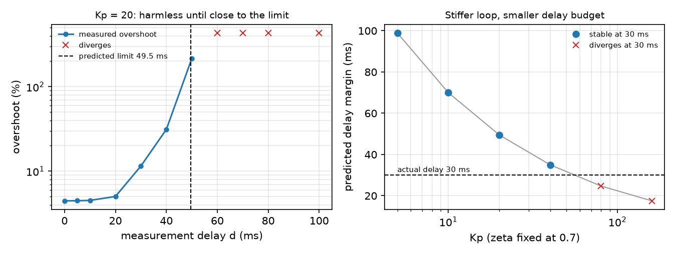
Left: overshoot versus delay, flat up to 20 ms, then rising steeply toward the predicted 49.5 ms limit. Right: delay margin falling as Kp rises at fixed damping ratio; the two stiffest gains drop below 30 ms and diverge.

Bisection on whole milliseconds: stable at 48 ms, unstable at 49 ms, oscillating with a period of 272 ms ( $2\pi/\omega_c$ = 273 ms). Up to about 20 ms the delay costs almost nothing; the last 20 ms before the limit cost everything.

B. Control rate. Same joint, no added delay, controller at $f$ Hz with zero-order hold (physics stays at 1 kHz). Second variant: the command is ready one tick later. Last two columns: part A at $T/2$ and $3T/2$ .

rate [Hz]	T [ms]	overshoot %	+ 1 tick compute	A at T/2	A at 3T/2
1000	1.0	4.45	4.46	4.45	4.46
100	10.0	4.48	4.61	4.47	4.62
50	20.0	4.55	10.31	4.51	11.51
30	33.3	4.75	78.07 (unstable)	4.72	215.84
20	50.0	5.34	diverges	6.66	diverges
10	100.0	diverges	diverges	215.84	diverges

The rules predict the trend: 30 Hz applied at once behaves like 17 ms of delay (fine), with one tick of compute like 50 ms (past the limit).

C. Prediction at $d$ = 40 ms (the predictor of Build it, Step 5):

controller	overshoot %	settle 2% [s]
no delay (reference)	4.45	0.398
delay, no prediction	31.23	0.926
delay + prediction, exact model	4.45	0.398
inertia +50% in the model	0.00	0.223
inertia −30% in the model	9.44	0.491
assumed delay 20 ms (true 40)	4.70	0.300

With an exact model and no disturbances, prediction removes the delay completely; a wrong model still helps here but changes the response. Knowing the delay and the dynamics (lesson 38) is what makes prediction safe.

D. SO-101 at 30 Hz. Menagerie SO-101, shoulder_pan servo (2 ms step). An outer “policy” loop at 30 Hz nudges the servo target from delayed readings: target += K*T*(goal - q_delayed), $K$ = 10 s⁻¹. For an ideal servo, this integrator with delay is unstable when $K(d + T/2) > \pi/2$ , above 140 ms (discrete-time analysis: from 5 ticks = 167 ms). The model servo is not ideal: alone, it reaches 50% of a 0.02 / 0.10 / 0.50 rad step after 18 / 44 / 110 ms, because it saturates on every step: with $k_p$ = 998 N·m/rad, 2.94/998 ≈ 3 mrad of error already demands its full 2.94 N·m, so a larger step takes longer.

delay [ms]	0	33	50	67	100	117	133
goal 0.1 rad: overshoot %	0.0	0.1	12.3	30.8	70.9	80.8	94.7
goal 0.1 rad: late \|e\|/goal	0.000	0.000	0.000	0.000	0.001	0.004	0.267
goal 0.5 rad: overshoot %	36.3	69.1	146.9	290.3	290.0	289.7	289.9
goal 0.5 rad: late \|e\|/goal	0.000	0.000	1.744	2.903	3.391	3.493	2.899

Small corrections keep oscillating only at 133 ms, near the ideal-servo estimate; a 0.5 rad move fails at 50 ms: the saturated servo adds its own, amplitude-dependent delay.

Break it

Fix the delay at 30 ms and make the PD loop stiffer at constant ζ = 0.7 (right panel of the figure above):

$K_p$	5	10	20	40	80	160
$\omega_c$ [rad/s]	11.49	16.25	22.99	32.51	45.97	65.01
$d_{\max}$ [ms]	98.9	70.0	49.5	35.0	24.7	17.5
overshoot %	4.73	5.30	11.51	37.78	diverges	diverges

The damping ratio is the same in every row, yet the loop dies at $K_p$ = 80: stiffness raises $\omega_c$ , and the same 30 ms costs $\omega_c d$ of phase. The formula predicts the failing rows exactly (24.7 and 17.5 ms are below 30 ms). Gains tuned in a zero-delay simulation are tuned for a loop that does not exist.

On the real robot

Measure the latency, do not guess it. LeRobot’s SO-101 follower times each bus and camera read in get_observation and logs them at debug level (so_follower.py). Procedure: command a step on one joint, log command and Present_Position time stamps, take the time until the reading moves. Not yet measured on the real arm.
The servo runs its own inner loop (part D): outer-loop latency costs reaction time, and stability when the policy reacts to its own delayed observations.
Simulate the latency you will have (Tan et al. did, with system identification and an actuator model): put the measured delay into the training simulator (lesson 39), for example with MuJoCo’s delay attribute.

Check yourself

Quick check · 2 questions. Click an answer.

1. Overshoot is 4.45% without delay, 5.02% at 20 ms and 31.23% at 40 ms; at 50 ms the loop is unstable. Why does it fail so abruptly?

The delay lowers the loop gain until the joint can no longer reach the target.
The 1 kHz physics step becomes too coarse beyond 40 ms.
The delay removes phase $\omega_c d$ at the crossover; once that eats the 65.2° phase margin, at $d_{\max} = 49.5$ ms, corrections reinforce the error.

Why: Part A: predicted 49.5 ms, measured stable at 48 ms and unstable at 49 ms, oscillating with the predicted period (272 ms vs 273 ms). A delay changes phase, not gain.

2. In Break it the delay is fixed at 30 ms and Kp is raised at the same damping ratio ζ = 0.7. Why does the loop diverge at Kp = 80?

A stiffer loop has a higher crossover frequency, so the same 30 ms costs more phase; its delay margin falls to 24.7 ms.
A higher Kp at constant ζ means less damping, so it overshoots more.
The torque limit is reached at Kp = 80.

Why: Break it table: $\omega_c$ 22.99 → 45.97 rad/s and $d_{\max}$ 49.5 → 24.7 ms from Kp 20 to 80; the formula predicts both failing rows (24.7 and 17.5 ms are below 30 ms).

Easy. A camera pipeline adds 40 ms, the policy runs at 20 Hz and its output is applied one tick after the frame. Estimate the total delay with the $T/2$ rule.
Medium. Using $d_{\max} = \mathrm{PM}/\omega_c$ , explain why part B’s 30 Hz loop with one tick of compute fails while part A at 40 ms survives.
Hard. In part C, replace the exact predictor’s model with one that ignores the motor command (pure extrapolation $q + \dot q\,d$ ). Predict, then run: overshoot at 40 ms?

Answers

40 ms + 50 ms (one tick of compute) + 25 ms (hold) = 115 ms.
One tick of compute plus hold at 30 Hz is about $3T/2$ = 50 ms, past the 49.5 ms margin; part A’s 40 ms is inside it (31.23% overshoot, stable).
15.15% overshoot, between exact prediction (4.45%) and none (31.23%), but settling takes 1.902 s (no prediction: 0.926 s): extrapolation ignores the acceleration the controller commanded during the delay. Row “extrapolation” in part C of output.txt.

Takeaways and sources

Delay removes phase $\omega d$ ; the loop survives up to $d_{\max} = \mathrm{PM}/\omega_c$ (predicted 49.5 ms, measured 48–49 ms, oscillating at the predicted 273 ms period).
Control rate adds about $T/2$ , plus $T$ per tick of compute: here 30 Hz is fine applied at once, unstable with one tick of compute.
Prediction with a correct model removes the delay (31.23% → 4.45%); stiffer loops and saturating actuators tolerate less.

Next: lesson 38 · System identification.

Sources:

LeRobot · Imitation learning on real-world robots (30 fps examples, lerobot-rollout, --inference.type=rtc; read 2026-10-27).
LeRobot configuration_act.py, so_follower.py (Apache-2.0).
J. Tan et al., Sim-to-Real: Learning Agile Locomotion For Quadruped Robots, 2018.
T. Zhao et al., Learning Fine-Grained Bimanual Manipulation with Low-Cost Hardware (ACT), 2023.
MuJoCo Menagerie · robotstudio_so101 (Apache-2.0).
Lynch & Park, Modern Robotics, ch. 11.
All measured numbers: experiments/37-latency/output.txt.