13 · Trajectory generation


Part	4 · Dynamics and control
Run type	CPU · Mac or Colab CPU
Prerequisites	10, 12
Learn first	Calculus for Machine Learning
Time	~45 min
Code	`experiments/13-trajectory-generation/experiment.py`
Status	✅ done

Act on this lesson

Tick each step when you have done it. Saved in this browser only.

01 · Read The problem and the core idea; answer the questions before you read.
02 · Build it Type the steps yourself, then run uv run python experiments/13-trajectory-generation/build.py
03 · Run the experiment Predict first, then run uv run python experiments/13-trajectory-generation/experiment.py
04 · Break it Change the one parameter and watch it fail.
05 · Check yourself Quizzes and exercises at the end.

A controller tracks whatever you give it. Give it a step and it will try to produce infinite acceleration; give it a smooth curve and the torque stays small.

The problem

In lesson 12, Unitree’s real-robot stand-up example did not send the stand pose in one go: it interpolated toward it in phases of 500 to 1000 ticks of 2 ms (go2_stand_example.py). Robot interfaces go further: libfranka’s rate_limiting.h defines per-joint maxima of 10 rad/s² acceleration, 5000 rad/s³ jerk (the rate of change of acceleration) and 1000 N·m/s torque rate at a 1 ms control period, with limitRate functions that clip commands to them (rate_limiting.h). A planner or an IK solver gives you where to go; trajectory generation decides how the reference moves in time, and that choice sets the peak torque, the jerk that shakes the structure, and the tracking error (how far the robot lags behind its reference). This lesson measures all three on a Panda.

Before you read · 2 questions. Guess first; the lesson tells you why.

1. You do the same quintic move in half the time. What happens to the reference’s peak acceleration and peak jerk?

Both double, because everything happens twice as fast.
Acceleration ×4, jerk ×8.
Neither changes; the shape alone fixes them.

Why: By the chain rule $\ddot q \propto 1/T^2$ and $\dddot q \propto 1/T^3$ . Part B, quintic from 1 s to 0.5 s - acceleration 3.46 → 13.86 rad/s², jerk 35.8 → 284.6 rad/s³.

2. Which elevator ride feels smoother: speed ramps up at a constant rate and down again, or the acceleration itself eases in and out?

The constant-rate ramp, because its acceleration is lower.
Both feel the same if they take the same time.
The one whose acceleration eases in: a jump in acceleration is the lurch you feel (jerk).

Why: In plain words: jerk is the rate of change of acceleration. The trapezoid’s acceleration jumps (robot jerk 1003 rad/s³), the quintic’s does not (35 rad/s³).

Core idea

In plain words

A controller chases its reference, the angle it is told to be at right now. If the reference teleports to the goal (a step), the controller tries to get there instantly and asks for an enormous torque. A trajectory is the reference written as a schedule instead: where each joint should be at every tick between start and goal.

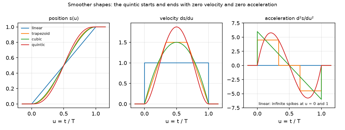
Think of an elevator. A cheap one lurches when it starts and stops; a good one eases into motion, cruises and eases out. What you feel as a lurch is jerk, the rate at which acceleration changes. The shape of the schedule decides it:

linear: constant speed from the first instant, so speed jumps at both ends;
trapezoid: speed ramps up, cruises, ramps down, so acceleration jumps at the corners;
cubic: speed is smooth, but acceleration still jumps at the start and the end;
quintic: position, speed and acceleration all start and end at rest. This is the minimum-jerk move.

Duration matters more than shape: do the same move in half the time and every acceleration (and torque) is four times larger, every jerk eight times. Two more choices: interpolate in joint angles (cheap, the hand follows a curve) or along a straight hand line (IK at every point), and whether to add feedforward, the torque the planned acceleration needs, sent in advance.

flowchart TD
    G["goal joint angles<br/>from a planner or IK"] --> TG["trajectory generator<br/>q_r(t) = q0 + s(t/T)·Δq"]
    TG --> R["q_r, q̇_r, q̈_r<br/>every 2 ms"]
    R --> PD["PD + gravity<br/>tracks q_r, q̇_r"]
    R --> FF["feedforward<br/>M(q)·q̈_r"]
    PD --> S["add, clip to torque limits"]
    FF --> S
    S --> A["Panda"]
    A -- "measured q, q̇" --> PD

Time scaling as code

Every move is “start + fraction of the way × total change”; only the fraction s changes with time.

u = min(max(t / T, 0.0), 1.0)                          # normalised time, 0 at start, 1 at the end
s, sd, sdd = quintic_s(u), quintic_s1(u) / T, quintic_s2(u) / T**2   # fraction done and its time derivatives
q_ref, qd_ref, qdd_ref = q0 + s*dq, sd*dq, sdd*dq      # per-joint reference [rad, rad/s, rad/s^2]
tau = g(q) + kp*(q_ref - q) + kd*(qd_ref - qd)         # PD tracking + gravity (lesson 12)
tau += M(q) @ qdd_ref                                  # optional feedforward (lesson 11's M)

| shape | $s(u)$ | boundary conditions | peak $|\ddot q|$ | jerk | |---|---|---|---|---| | step | 1 | none | ∞ | ∞ | | linear | $u$ | position | ∞ (velocity jumps) | ∞ | | trapezoidal velocity | accelerate $T/3$ , cruise, decelerate $T/3$ | position, velocity | $4.5\,\Delta q/T^2$ | ∞ (acceleration jumps) | | cubic | $3u^2 - 2u^3$ | position, velocity | $6\,\Delta q/T^2$ | ∞ at the ends | | quintic | $10u^3 - 15u^4 + 6u^5$ | position, velocity, acceleration | $5.77\,\Delta q/T^2$ | $60\,\Delta q/T^3$ |

Here $q(t) = q_0 + s(t/T)\,\Delta q$ , $u = t/T \in [0,1]$ is normalised time, $s(u)$ the time scaling with $s(0) = 0$ and $s(1) = 1$ (Lynch & Park, ch. 9), $q_0$ the start angles, $\Delta q$ the total change, $T$ the duration, $\ddot q$ the joint acceleration and jerk $\dddot q$ its time derivative. “Boundary conditions” lists what the shape sets to rest at both ends.

Position, velocity and acceleration of the linear, trapezoid, cubic and quintic time scalings over normalised time. Only the quintic starts and ends with both zero velocity and zero acceleration; the cubic's acceleration jumps to 6 at the ends, the trapezoid's jumps at its corners.

Joint space vs Cartesian. Joint-space interpolation stays inside the joint limits whenever both ends do, but the hand follows a curve. A Cartesian line needs IK at every waypoint (lesson 10) and can meet singularities or joint limits.

Feedforward. A tracking controller $\tau = g(q) + K_p(q_r - q) + K_d(\dot q_r - \dot q)$ produces torque only from an error. Adding the model term $M(q)\ddot q_r$ (lesson 11) supplies the accelerating torque in advance; a smooth reference makes $\ddot q_r$ available and bounded.

Math details: where the quintic comes from, and the 1/T² and 1/T³ laws

Polynomials from boundary conditions. A cubic has four coefficients, enough for $s$ and $\dot s$ at both ends: $s(0)=0$ , $s(1)=1$ , $s'(0)=s'(1)=0$ give $3u^2 - 2u^3$ . Its acceleration $s'' = 6 - 12u$ is $\pm 6$ at the ends, and jumps there from the zero of the rest state. A quintic has six coefficients; adding $s''(0) = s''(1) = 0$ gives $10u^3 - 15u^4 + 6u^5$ . Its acceleration $s'' = 60u - 180u^2 + 120u^3$ peaks at $u = (3-\sqrt3)/6$ with value $10\sqrt3/3 \approx 5.77$ ; its jerk $s''' = 60 - 360u + 360u^2$ is largest at the ends, 60.

Minimum jerk. Minimising $\int_0^1 (s''')^2\,du$ gives, by the Euler–Lagrange equation, $s^{(6)} = 0$ : a fifth-order polynomial. With rest at both ends it is exactly the quintic above (Flash & Hogan 1985).

Scaling with duration. By the chain rule, $\dot q = \Delta q\, s'(u)/T$ , $\ddot q = \Delta q\, s''(u)/T^2$ , $\dddot q = \Delta q\, s'''(u)/T^3$ . The shape fixes the constants in the table; the duration fixes the powers of $T$ . Joint torque $\approx M\ddot q$ + gravity, so halving $T$ quadruples the dynamic part of the torque.

Why a jump means infinite jerk. If acceleration changes by a finite amount in zero time, its derivative is a spike (in a 2 ms simulation: the change divided by 2 ms), which is what the robot-jerk columns of the experiment measure.

Go deeper: Calculus for Machine Learning (derivatives, chain rule); Lynch & Park, Modern Robotics, ch. 9; T. Flash, N. Hogan, doi:10.1523/JNEUROSCI.05-07-01688.1985.

Build it

You will now write the time scalings yourself in about 40 lines of NumPy, derive the polynomials instead of copying them, and check every number of the formula table, then track the result on the Experiment’s Panda with lesson 11’s mass matrix.

Type the steps into a file of your own (for example scratch/my_trajectory.py) and run it after each step. The finished functions are in physai/trajectory.py; uv run python experiments/13-trajectory-generation/build.py runs all five steps with the checks (output in build_output.txt).

Step 1 · Polynomials from boundary conditions

Each condition “the $r$ -th derivative at $u$ equals $v$ ” is one linear equation in the coefficients, because $\frac{d^r}{du^r}u^k = \frac{k!}{(k-r)!}u^{k-r}$ . As many conditions as coefficients, one solve:

def poly_from_boundary(conds, degree):
    """Coefficients c (s = sum_k c_k u^k) that meet every condition (u, derivative order, value)."""
    A = [[factorial(k) / factorial(k - r) * u ** (k - r) if k >= r else 0.0 for k in range(degree + 1)]
         for u, r, _ in conds]
    return np.linalg.solve(np.array(A), np.array([v for _, _, v in conds], dtype=float))

def poly_eval(c, u, order=0):
    """The order-th derivative of the polynomial with coefficients c, at u."""
    return P.polyval(u, P.polyder(c, order))

REST = [(0, 0, 0.0), (1, 0, 1.0), (0, 1, 0.0), (1, 1, 0.0)]      # s(0) = 0, s(1) = 1, at rest at both ends
CUBIC = poly_from_boundary(REST, 3)
QUINTIC = poly_from_boundary(REST + [(0, 2, 0.0), (1, 2, 0.0)], 5)  # ... and zero acceleration at both ends

== Step 1. Coefficients from boundary conditions (c0 + c1 u + c2 u^2 + ...) ==
cubic   (s, s' at both ends):          0.00   0.00   3.00  -2.00
quintic (s, s', s'' at both ends):     0.00   0.00   0.00  10.00 -15.00   6.00
max diff to 3u^2 - 2u^3: 0.0e+00, to 10u^3 - 15u^4 + 6u^5: 1.1e-14
one more pair (zero jerk at both ends) gives degree 7: 0 0 0 0 35 -84 70 -20

The textbook polynomials fall out, and one more pair of conditions gives the next member of the family ( $35u^4 - 84u^5 + 70u^6 - 20u^7$ , zero jerk at the ends too).

Step 2 · Derivatives and peaks

Each shape returns $s$ , $s'$ and $s''$ on normalised time:

def cubic(u):
    """Cubic time scaling 3u^2 - 2u^3: s, ds/du, d2s/du2."""
    return poly_eval(CUBIC, u), poly_eval(CUBIC, u, 1), poly_eval(CUBIC, u, 2)

def quintic(u):
    """Quintic (minimum-jerk) time scaling 10u^3 - 15u^4 + 6u^5: s, ds/du, d2s/du2."""
    return poly_eval(QUINTIC, u), poly_eval(QUINTIC, u, 1), poly_eval(QUINTIC, u, 2)

== Step 2. Peaks of the normalised shapes (100001 points on [0, 1]) ==
   shape  max ds/du  max d2s/du2    at u  max |d3s/du3| inside
   cubic     1.5000       6.0000  0.0000               12.0000
 quintic     1.8750       5.7735  0.2113               60.0000
formulas: cubic 1.5, 6 at u = 0; quintic 1.875, 10 sqrt(3)/3 = 5.7735 at u = (3 - sqrt(3))/6 = 0.2113, jerk 60

Every value matches the closed forms of the math details: the cubic’s acceleration peaks at the ends (6), the quintic’s at $u = 0.2113$ ( $10\sqrt3/3$ = 5.7735), and the quintic’s jerk is 60 at the ends. The cubic’s jerk is a constant 12 inside, but its acceleration jumps from 0 to 6 at $u = 0$ : that jump is the ”∞” in the table.

Step 3 · The trapezoid

The trapezoid is piecewise: a parabola, a straight line, a parabola. Its acceleration $a$ follows from $s(1) = 1$ :

def trapezoid(u, ta=1 / 3):
    """Trapezoidal velocity: accelerate for ta, cruise, decelerate for ta. Returns s, ds/du, d2s/du2."""
    a = 1 / (ta * (1 - ta))                        # the acceleration that makes s(1) = 1
    if u < ta:
        return 0.5 * a * u ** 2, a * u, a
    if u <= 1 - ta:
        return 0.5 * a * ta ** 2 + a * ta * (u - ta), a * ta, 0.0
    return 1 - 0.5 * a * (1 - u) ** 2, a * (1 - u), -a

== Step 3. The trapezoid (ta = 1/3) ==
s(1) = 1.000000, peak ds/du = 1.5000, peak |d2s/du2| = 4.5000
max |s - integral of ds/du| = 1.0e-10 (s is continuous; d2s/du2 jumps 0 -> 4.5)

Step 4 · From shape to joint reference

The chain rule turns $s(u)$ into a joint reference: divide by $T$ for each derivative. Outside the move the reference is at rest:

def joint_reference(shape, t, T, q0, dq):
    """Reference angle, speed and acceleration at time t of the move q0 -> q0 + dq lasting T seconds."""
    s, s1, s2 = shape(min(max(t / T, 0.0), 1.0))
    if not 0.0 < t < T:                            # at rest before and after the move
        s1 = s2 = 0.0
    return q0 + s * dq, s1 / T * dq, s2 / T ** 2 * dq

== Step 4. Reference peaks of the Panda move (largest joint 0.6 rad) ==
 T (s)     shape  exact acc  2 ms acc  exact jerk  2 ms jerk
  0.25     cubic      57.60     56.68         inf        inf
  0.25   quintic      55.43     55.41     2304.00    2249.00
  0.50     cubic      14.40     14.28         inf        inf
  0.50   quintic      13.86     13.86      288.00     284.55
  1.00     cubic       3.60      3.59         inf        inf
  1.00   quintic       3.46      3.46       36.00      35.78
  2.00     cubic       0.90      0.90         inf        inf
  2.00   quintic       0.87      0.87        4.50       4.49
  1.00 trapezoid       2.70      2.70

The “exact” columns are the formula table times 0.6 rad: $1/T^2$ for acceleration, $1/T^3$ for jerk. The Experiment’s table holds the “2 ms” columns, because it samples the reference at the control rate and counts it as at rest at $t = 0$ : the cubic’s first sample is at 2 ms, where $s'' = 6 - 12 \cdot 0.002$ , hence 3.59 instead of 3.60, and the quintic’s jerk is a 2 ms finite difference, 35.78 instead of 36.00. At T = 0.25 s the gaps grow (56.68 vs 57.60, 2249.00 vs 2304.00) because 2 ms is then a larger share of the move.

Step 5 · Track it, with your own feedforward

Feed joint_reference to the Experiment’s controller and add $M(q)\ddot q_r$ with mass_matrix from lesson 11:

q_ref, qd_ref, qdd_ref = joint_reference(quintic, d.time, 1.0, Q0, DQ)
tau = d.qfrc_bias[:7] + KP * (q_ref - d.qpos[:7]) + KD * (qd_ref - d.qvel[:7])
tau = tau + mass_matrix(tree, d.qpos)[:7, :7] @ qdd_ref - d.qfrc_passive[:7]   # feedforward

== Step 5. Track the quintic on the Panda (T = 1 s, the Experiment's PD + qfrc_bias) ==
PD + gravity              tracking error 1.32 deg, robot peak jerk 35 rad/s^3
PD + M qdd_ref - passive  tracking error 0.01 deg, robot peak jerk 48 rad/s^3

The Experiment’s quintic rows, 1.32° and 0.01°, from your reference and your mass matrix.

What you keep

physai.trajectory now has poly_from_boundary, poly_eval, cubic, quintic, trapezoid and joint_reference. Lesson 14 ramps its contact target with the same quintic. tests/test_13_trajectory_generation.py checks them against the closed forms; run uv run pytest tests/test_13_trajectory_generation.py after you change anything.

Use it

MuJoCo has no trajectory generator: it simulates whatever reference you compute. For a point-to-point move, SciPy’s splines give the same curves:

from scipy.interpolate import CubicSpline, make_interp_spline

cs = CubicSpline([0, T], [q0, q1], bc_type="clamped")              # zero speed at both ends: the cubic
qs = make_interp_spline([0, T], [q0, q1], k=5,
                        bc_type=([(1, 0.0), (2, 0.0)], [(1, 0.0), (2, 0.0)]))   # + zero acceleration: the quintic
q, qd, qdd = qs(t), qs(t, 1), qs(t, 2)

== Use it. SciPy splines through the two end points (T = 1 s, 0 -> 0.6 rad) ==
CubicSpline(bc_type='clamped') vs cubic: max diff 3.3e-16 rad
make_interp_spline(k=5, zero speed and acceleration) vs quintic: max diff 1.5e-15 rad, peak jerk 36.00 rad/s^3

With more than two points the same calls give a smooth curve through all waypoints, which the single-move formulas cannot.

Tool	Call	Shape
physai	`joint_reference(quintic, t, T, q0, dq)`	$q$ , $\dot q$ , $\ddot q$ at time $t$
SciPy	`CubicSpline(t, q, bc_type="clamped")`, `make_interp_spline(t, q, k=5, bc_type=...)`	piecewise polynomials through waypoints; `spline(t, n)` gives the $n$ -th derivative
Modern Robotics code	`CubicTimeScaling(Tf, t)`, `QuinticTimeScaling(Tf, t)`, `JointTrajectory(thetastart, thetaend, Tf, N, method)`	$s(t)$ only, and $N$ sampled joint vectors (`core.py`)
libfranka	`limitRate(...)`	clips commanded velocity, acceleration and jerk to the robot’s limits (`rate_limiting.h`)

Three traps:

Normalised vs real time. $s'(u)$ is per unit of $u$ ; the joint speed is $s'(u)\,\Delta q / T$ . Forgetting one $1/T$ is the most common bug, and at T = 0.25 s it is a factor of 4.
Sampled peaks are not peaks. A reference checked against a limit at the control rate can miss a jump that happens between samples (Step 4: 3.59 vs 3.60).
Clamping is not smoothing. A rate limiter keeps each command legal but turns a jumpy reference into a different, unplanned motion; plan a smooth one instead.

Check after building · 2 questions.

1. How does Build it, Step 1 get the quintic’s coefficients?

From six boundary conditions (s, s’, s” at both ends), one linear equation each, solved together.
By fitting a polynomial to the Experiment’s measured joint angles.
By integrating the cubic once more.

Why: poly_from_boundary returns 0, 0, 0, 10, −15, 6; one more pair (zero jerk) gives the degree-7 shape 35u⁴ − 84u⁵ + 70u⁶ − 20u⁷.

2. The formula gives the cubic’s peak acceleration at T = 1 s as 3.60 rad/s², the Experiment’s table 3.59. Why (Build it, Step 4)?

The Panda’s torque limits cut the acceleration.
The Experiment samples the reference every 2 ms and counts it as at rest at t = 0, so its first sample is at 2 ms, where s” = 6 − 12·0.002.
The cubic’s coefficients are rounded in the Experiment.

Why: Same reason for the quintic’s jerk, 35.78 instead of 36.00: a 2 ms finite difference. At T = 0.25 s the gap grows (56.68 vs 57.60).

Experiment

Setup. Panda (Menagerie) from the home keyframe, joint move $\Delta q$ = (0.6, 0.4, −0.4, 0.5, 0.5, −0.4, 0.6) rad. The model’s built-in position actuators are switched off (actuator_gainprm and actuator_biasprm set to 0) and torques go to qfrc_applied, clipped at the model’s limits (87 N·m joints 1–4, 12 N·m joints 5–7). Controller and physics run at 2 ms:

s, sd, sdd = profile(kind, d.time, T)
q_ref, qd_ref = Q0 + s * DQ, sd * DQ
tau = d.qfrc_bias[:7] + KP * (q_ref - q) + KD * (qd_ref - qd)    # PD + gravity/Coriolis
tau = np.clip(tau, -lim, lim)

Kp = (600, 600, 600, 600, 250, 150, 50), Kd = (50, 50, 50, 50, 20, 12, 4). “Robot” columns are measured from qacc in simulation; robot jerk is its finite difference at 2 ms. “Steps saturated” is the share of control steps in which some joint torque was clipped at its limit. Full script: experiments/13-trajectory-generation/experiment.py. MuJoCo 3.17.0, NumPy 2.5.4, Python 3.14, Apple M5, deterministic, ~4 s.

Predict. Which shape has the smallest tracking error? Which has the smallest jerk?

A. Five shapes, T = 1 s (reference values for the largest joint, 0.6 rad; errors = max $|q_r - q|$ during the move):

shape	ref. peak acc [rad/s²]	ref. peak jerk [rad/s³]	robot peak acc	robot peak jerk	tracking error	steps saturated
step	∞	∞	739.2	175025	34.35°	5.5%
linear	∞	∞	220.9	110475	0.78°	0.0%
trapezoid	2.70	∞	3.0	1003	1.08°	0.0%
cubic	3.59	∞	3.6	1337	1.05°	0.0%
quintic	3.46	35.78	3.7	35	1.32°	0.0%
quintic + $M\ddot q_r$ − passive	3.46	35.78	3.5	48	0.01°	0.0%

The step saturates the torque in 5.5% of steps and lags 34.35° behind its own reference; the robot’s acceleration peaks at 739.2 rad/s².
Jerk follows continuity. Every shape whose acceleration jumps (linear, trapezoid, cubic) produces robot jerk of 1003–110475 rad/s³; the quintic produces 35 rad/s³, matching its reference (35.78). Jerk is what excites flexible links, gearboxes and the object in the gripper.
The tracking error of smooth shapes is about 1° and not decided by the shape. The worst joint is joint 7 (Kp 50), where the model’s passive damping (1 N·m·s/rad) and the inertia are not compensated. Adding the model feedforward $M\ddot q_r$ and cancelling qfrc_passive drops the error to 0.01°. The shape decides jerk; the model decides tracking error.

B. Sweep the duration (same move):

T [s]	shape	ref. peak acc	ref. peak jerk	robot peak jerk	error
0.25	cubic	56.68	∞	21311	4.46°
0.25	quintic	55.41	2249.0	2107	5.52°
0.50	cubic	14.28	∞	5317	2.16°
0.50	quintic	13.86	284.6	234	2.73°
1.00	cubic	3.59	∞	1337	1.05°
1.00	quintic	3.46	35.8	35	1.32°
2.00	cubic	0.90	∞	335	0.52°
2.00	quintic	0.87	4.5	4	0.65°

Acceleration scales as $1/T^2$ (56.68 → 14.28 → 3.59 → 0.90, factor 4 per halving), the quintic’s jerk as $1/T^3$ (2249.0 → 284.6 → 35.8 → 4.5, factor 8), and the PD-only tracking error roughly as $1/T$ . At every duration the cubic’s robot jerk is an order of magnitude or more above the quintic’s (21311 vs 2107 rad/s³ at 0.25 s, 335 vs 4 at 2 s).

C. Joint space vs Cartesian. The tool centre point moves 50 cm along $y$ with constant orientation, between IK solutions A and B (IK residual below 0.001 mm):

interpolation	max distance from the line	hand path	joint path
joint space (quintic in $q$ )	5.38 cm	51.53 cm	1.089 rad
Cartesian (IK per waypoint)	0.00 cm	50.00 cm	1.256 rad

Same endpoints, same timing: the joint-space path bows 5.38 cm off the line. Enough to hit a box edge in a cluttered scene; irrelevant in free space, where joint space is cheaper (1.089 vs 1.256 rad of joint travel) and never meets a singularity mid-path.

Break it

Shorten the move. At T = 0.25 s the reference needs 55.41 rad/s² (quintic) on a 0.6 rad joint motion; even the smooth quintic now produces 2107 rad/s³ of robot jerk and 5.52° of tracking error. Go to the extreme, T → 0, and you get the step: torque saturation (5.5% of steps), 739.2 rad/s² acceleration and a 34.35° lag. The mechanism is the scaling law, not the controller: no gain setting can produce acceleration the actuators cannot supply, and when the torque clips, the PD’s carefully tuned damping is gone.

On the real robot

Panda / FR3 class. libfranka’s rate limiter constants (10 rad/s² joint acceleration, 5000 rad/s³ jerk, 1 ms period; rate_limiting.h) are violated by any reference that jumps. In our sweep, both cubic and quintic exceed 10 rad/s² at T = 0.5 s (14.28 and 13.86), and the cubic’s acceleration discontinuity gives unbounded jerk at any duration. A quintic of 1 s stays inside both limits (3.46 rad/s², 35.78 rad/s³). These comparisons use our simulated references; nothing here was run on a Panda.
Go2. The SDK stand example’s piecewise-linear ramp (lesson 12) is the “linear” row: bounded position steps, but velocity jumps at every waypoint.
SO-101. The servos receive goal positions at the rate of the control loop. A policy running at 30 Hz that outputs raw targets is effectively sending a staircase; whether interpolating between targets reduces jerk on the real arm is not yet measured.

Check yourself

Quick check · 2 questions. Click an answer.

1. The trapezoid has the lowest reference peak acceleration (2.70 rad/s²) at T = 1 s. Why does the Panda still see far more jerk with it than with the quintic?

Its acceleration jumps at the corners; only the quintic starts and ends with zero acceleration.
Its cruise phase is too fast for the PD gains.
It saturates the joint torques, like the step.

Why: Jerk follows continuity of acceleration - part A measures 1003 rad/s³ robot jerk for the trapezoid vs 35 for the quintic, with 0.0% saturated steps for both.

2. All smooth shapes track with about 1° of error at T = 1 s. What brought the quintic’s error down to 0.01°?

Switching from the cubic to the quintic.
Making the move twice as long.
Adding the model feedforward $M\ddot q_r$ and cancelling qfrc_passive.

Why: The shape decides jerk, the model decides tracking error. Part A - quintic 1.32°, quintic + feedforward 0.01°; doubling T only reaches 0.65° (part B).

Easy. A quintic moves a joint 1 rad in 2 s. What are its peak acceleration and peak jerk?
Medium. Why does the linear profile have the smallest tracking error in part A (0.78°) despite an infinite reference acceleration?
Hard. Add $M(q)\ddot q_r -$ qfrc_passive feedforward to the cubic and the trapezoid in experiment.py. Predict before running: does their tracking error also drop to ~0.01°? Does their robot jerk change?

Answers

Peak acceleration $5.77 \cdot 1 / 2^2 \approx 1.44$ rad/s²; peak jerk $60 \cdot 1 / 2^3 = 7.5$ rad/s³ (formulas from the table).
Its peak velocity ( $\Delta q/T$ ) is the lowest of all shapes and its acceleration is zero except for two instants, which is consistent with the unmodelled damping torque being smallest; the infinite acceleration only appears as two short spikes (220.9 rad/s² robot peak) at the start and end.
Not computed here; run it.

Takeaways and sources

Time scaling sets the physics: accelerations scale with $1/T^2$ , jerks with $1/T^3$ ; a step saturates the Panda’s torque and lags 34.35°.
Continuity of acceleration decides jerk: quintic 35 rad/s³ vs 1003–1337 rad/s³ for trapezoid and cubic at T = 1 s. Tracking error is decided by the model: feedforward cuts it from 1.32° to 0.01°.
Joint-space interpolation bows off the straight line (5.38 cm over 50 cm here); use Cartesian interpolation only where the path matters.

Next: lesson 14 · Operational-space and impedance control.

Sources:

Lynch & Park, Modern Robotics, ch. 9 (Trajectory Generation).
T. Flash, N. Hogan, “The coordination of arm movements: an experimentally confirmed mathematical model”, Journal of Neuroscience 5(7):1688–1703, 1985, doi:10.1523/JNEUROSCI.05-07-01688.1985.
libfranka rate_limiting.h (main branch, read 2026-10-27); go2_stand_example.py.
MuJoCo Menagerie · franka_emika_panda.
All measured numbers: experiments/13-trajectory-generation/output.txt.