34 · Observation and action design


Part	8 · Reinforcement learning for robots
Run type	CPU · Mac or Colab CPU
Prerequisites	33
Learn first	Proximal Policy Optimization (PPO)
Time	~60 min
Code	`experiments/34-observation-action-design/experiment.py`
Status	✅ done

Act on this lesson

Tick each step when you have done it. Saved in this browser only.

01 · Read The problem and the core idea; answer the questions before you read.
02 · Build it Type the steps yourself, then run uv run python experiments/34-observation-action-design/build.py
03 · Run the experiment Predict first, then run uv run python experiments/34-observation-action-design/experiment.py
04 · Break it Change the one parameter and watch it fail.
05 · Check yourself Quizzes and exercises at the end.

The policy does not move the robot. It talks to a controller, and what its numbers mean decides most of what it can learn.

The problem

Unitree’s Go2 policy does not output torques. Its 12 outputs are scaled by 0.25, added to a default joint angle, and tracked by a PD loop that runs four times per policy step (go2_config.py, legged_robot.py · _compute_torques):

torques = self.p_gains*(actions_scaled + self.default_dof_pos - self.dof_pos) - self.d_gains*self.dof_vel

with stiffness = 20, damping = 0.5, action_scale = 0.25, decimation = 4 at dt = 0.005 (50 Hz policy, 200 Hz PD). Why this and not torques, and why those numbers? With the PPO of lesson 33 held fixed, we change only the interface on the SO-101 reach and measure success, smoothness and energy.

Before you read · 2 questions. Guess first; the lesson tells you why.

1. Giving the policy the absolute target position instead of target − gripper took success from 298/300 to 101/300. Why?

To know which way to move, the policy now has to learn forward kinematics itself.
The absolute position is a longer vector, so the network is too small.
The absolute position is measured with more noise.

Why: Section C, observation table. The relative goal is the single most important input; the Go2 observation is built the same way, in the frame the policy acts in.

2. A policy outputs raw joint torques at 50 Hz instead of joint targets for a servo. What extra work does it take on?

None; a torque and a target are the same command.
Only the inverse kinematics.
Everything the servo’s fast loop did, holding the arm against gravity and damping its motion, at 50 Hz instead of the physics rate.

Why: Plain words and Math details; with targets the PD loop runs every 5 ms physics step. In section A torques reached 272/300 against 298/300 for absolute targets (overlapping only with delta targets).

Core idea

In plain words

The policy is a slow, high-level service that calls a fast, low-level one, in one of three ways. Torque: write the motor effort directly, like poking hardware registers; the policy must then hold the arm against gravity and damp its motion itself. Absolute target: send the joint angle it wants; a PD loop (a spring-and-damper controller, lesson 12) chases that angle hundreds of times per second. Delta target: nudge the previous target by a small step.

With targets, the policy moves a setpoint 50 times per second and the stiff loop underneath does the rest. Three more choices sit around that call: the action scale (how far one unit of output reaches, and how large the exploration noise is in radians), the policy rate and the observation (“the target is a bit to the left of my gripper” is easier to act on than room coordinates).

From policy to torque

flowchart TD
    O["observation<br/>q, q̇, target − gripper, previous action"] --> P["policy, 50 Hz<br/>a in [-1, 1]"]
    P --> S["scale and offset<br/>q* = q0 + s·a"]
    S --> D["PD loop, every physics step<br/>τ = Kp (q* − q) − Kd q̇"]
    D --> L["clip to ±τmax"]
    L --> R["robot joints"]
    R --> O
    P -. "torque mode:<br/>τ = τmax · a" .-> L

The three interfaces, as code

def torque(a, q, qd, q_star_prev, mode, s):
    # a: policy output in [-1, 1]^4, q / qd: joint angles / velocities, s: action scale
    if mode == "torque":
        return TAU_MAX * a                          # policy is the controller; held for k physics steps
    if mode == "absolute":
        q_star = Q0 + s * a                         # setpoint around the default pose q0
    else:                                           # "delta"
        q_star = q_star_prev + s * a                # move the previous setpoint
    return clip(KP * (q_star - q) - KD * qd, -TAU_MAX, TAU_MAX)   # PD, every physics step

gamma = 1 - policy_dt / 0.4                         # keep a 0.4 s horizon when the rate changes

Name	Policy output means	Torque at every physics step
torque	$\tau = \tau_{\max} a$	held for $k$ steps
absolute target	$q^* = q_0 + s\,a$	$\tau = K_p (q^* - q) - K_d \dot q$ , clipped
delta target	$q^_t = q^_{t-1} + s\,a_t$	same PD

$a \in [-1,1]^n$ is the policy output, $q$ and $\dot q$ the joint angles and velocities, $q^*$ the joint target, $q_0$ the default pose, $s$ the action scale, $K_p$ and $K_d$ the PD gains, $\tau_{\max}$ the torque limit and $k$ the number of $h = 5$ ms physics steps per policy step.

Math details: what the servo, the scale, the rate and the observation do

The SO-101 servo is already a PD loop. Each STS3215 is a MuJoCo position actuator with kp = 998.22, kv = 2.731, forcerange = ±2.94 N·m; MuJoCo evaluates it inside every physics step (XML reference, actuators). Our torque mode removes that loop and drives the actuators as motors ( $\tau_{\max} = 2.94$ N·m). With targets, gravity and damping are handled at the physics rate; with torques the policy handles them at 50 Hz, with its noise in N·m.

Action scale. $s$ sets two things at once: the reachable range ( $q_0 \pm s$ ) and the size of exploration noise in physical units (the initial policy std $e^{-1} \approx 0.37$ becomes $0.37\,s$ rad). The Go2 uses $s = 0.25$ rad; a gait stays near the default pose, an arm reaching across its workspace does not.

Policy rate. $\Delta t = k h$ . A faster policy reacts sooner, but each decision matters less, and its discount must change to keep the same horizon in seconds (lesson 33): we set $\gamma = \lambda = 1 - \Delta t / 0.4\,\text{s}$ .

Observation. The Go2 policy sees 48 numbers (legged_robot.py · compute_observations): base linear and angular velocity, projected gravity, the velocity command, joint positions relative to the default, joint velocities and the previous action, each with a fixed scale. Our reach observation has the same structure: $q - q_0$ , $0.1\,\dot q$ , $p_{\text{target}} - p_{\text{gripper}}$ , previous action. We test two changes: dropping velocities, and giving the target as an absolute position instead of relative to the gripper.

Go deeper: Proximal Policy Optimization (PPO); MuJoCo · actuators; legged_robot.py.

Build it

You will now write the interface between policy and robot: the action map, the servo’s PD law, the decimation loop with its meters, and what changes with the control rate. Each step is checked against MuJoCo or the lesson’s ReachEnv; nothing is trained, and the script runs in about 3 s.

The functions are in physai/rl.py; uv run python experiments/34-observation-action-design/build.py runs the five steps (output in build_output.txt).

Step 1 · From policy output to actuator command

def action_to_ctrl(a, mode, q_home, scale, ctrl_prev, lo, hi, tau_max=2.94):
    """Map a policy output in [-1, 1] to the actuator command: absolute target, delta target or torque."""
    a = np.clip(a, -1.0, 1.0)
    if mode == "position":
        return np.clip(q_home + scale * a, lo, hi)
    if mode == "delta":
        return np.clip(ctrl_prev + scale * a, lo, hi)
    return tau_max * scale * a                                         # "torque": the policy is the controller

The check drives ReachEnv in each mode with random actions slightly outside $[-1, 1]$ and compares its command with yours:

== Step 1. Policy output -> actuator command, 3 episodes of random actions per mode ==
position (scale 1.0): max |ours - ReachEnv's command| = 0.0e+00
   delta (scale 0.1): max |ours - ReachEnv's command| = 0.0e+00
  torque (scale 1.0): max |ours - ReachEnv's command| = 0.0e+00

Step 2 · What the servo does with a target

def pd_torque(q_star, q, qd, kp, kd, tau_max):
    """What a position servo does at every physics step: a PD law towards the target, clipped to its torque limit."""
    return np.clip(kp * (q_star - q) - kd * qd, -tau_max, tau_max)

Read the gains from the model, put the arm in 1000 random states with targets about 3 mrad away, and compare with the force MuJoCo computes:

== Step 2. The servo's PD law vs MuJoCo, 1000 random states ==
STS3215 in the Menagerie model: kp = 998.22 N m/rad, kv = 2.731 N m s/rad, force range +-2.94 N m
max |ours - data.actuator_force| = 3.2e-13 N m; 1885 of 4000 torques at the limit
a position error of 2.95 mrad alone saturates the servo (2.94 / 998.22)

Your PD law is MuJoCo’s position actuator (3.2e-13 N·m). With kp = 998.22 a target 2.95 mrad away already demands the full 2.94 N·m, so 1885 of the 4000 torques sit at the limit: the stiffness the Experiment’s torque-rate column measures.

Step 3 · Decimation, and the two meters

The policy’s command is held while the physics runs $k$ steps; the meters sample at the physics rate:

def torque_rate_and_power(tau, qd, h):
    """Smoothness and energy of one episode at the physics rate.

    tau: (N + 1, n) actuator torques, starting with the one before the first step; qd: (N, n) joint velocities
    after each step; h: physics time step. Returns (RMS of ||d tau / dt|| [N m/s], mean sum |tau qdot| [W]).
    """
    rate = np.diff(tau, axis=0) / h
    return np.sqrt(np.mean(np.sum(rate ** 2, axis=1))), np.mean(np.sum(np.abs(tau[1:] * qd), axis=1))

for _ in range(own.frame_skip):                             # the command is held for k physics steps
    mujoco.mj_step(own.model, own.data)
    taus.append(own.data.actuator_force[own.act].copy())
    qds.append(own.data.qvel[own.vadr].copy())

== Step 3. Decimation and the physics-rate recorder: one episode per mode (position: scripted IK; torque: a = 0.1) ==
position: 320 physics steps; torque rate    345.9 N m/s (ReachEnv    345.9), power  1.713 W (ReachEnv  1.713)
  torque: 320 physics steps; torque rate      6.6 N m/s (ReachEnv      6.6), power  0.138 W (ReachEnv  0.138)

Your loop and meters reproduce ReachEnv’s recorder in both modes. One scripted-IK reach already shows Experiment A’s gap: 345.9 N·m/s through the stiff servo, 6.6 N·m/s for a constant torque.

Step 4 · The control rate changes the discount and the experience

def discount_for_rate(dt, horizon_s=0.4):
    """The discount that keeps a fixed look-ahead in seconds when the policy period dt changes."""
    return 1.0 - dt / horizon_s

== Step 4. Policy rate: gamma = 1 - dt / 0.4 s, and 300,000 policy steps in simulated time ==
frame_skip  rate Hz   gamma   simulated time
         1    200.0  0.9875       25 min
         2    100.0  0.9750       50 min
         4     50.0  0.9500      100 min
         8     25.0  0.9000      200 min
        16     12.5  0.8000      400 min

These are part B’s $\gamma$ column; the last column is its confound: 300,000 policy steps are 25 min of simulated time at 200 Hz, 100 min at 50 Hz, 400 min at 12.5 Hz.

Step 5 · The action scale decides what is reachable

Send the scripted IK controller through the same clipped interface at both scales, on the evaluation seeds:

== Step 5. Action scale: scripted IK through the same clipped interface, 100 episodes (seeds 10000-10099) ==
scale 1.00 rad: reaches 100/100
scale 0.25 rad: reaches 27/100
joint vectors drawn by the target sampler that lie within q0 +- 0.25 rad on all 4 joints: 1.8 %

100/100 at 1.0 rad, 27/100 at 0.25 rad: Break it’s reference numbers. Of the joint vectors the target sampler draws, only 1.8% lie inside $q_0 \pm 0.25$ rad on all four joints ( $0.25 \cdot (0.25/0.6)^3$ ); the IK reaches more (27%) because other joint combinations reach some of the same points, but most targets are outside the action space whatever the policy learns.

What you keep

physai.rl now also has action_to_ctrl, pd_torque, torque_rate_and_power and discount_for_rate. Lesson 36 uses the same PD-target interface on the Go2, and lesson 37 adds a delay between command and actuator. tests/test_34_observation_action_design.py checks the modes, the PD law against MuJoCo and the meters on a hand example; run uv run pytest tests/test_34_observation_action_design.py.

Use it

In MuJoCo the interface is chosen in the model, not in Python: a <position> actuator with kp and kv is the PD servo of Step 2, a <motor> is a plain torque, and forcerange is the clip (XML reference, actuators). The lesson’s torque mode rewrites the model’s gain and bias parameters to turn the servos into motors (in ReachEnv.__init__). Unitree’s training code instead computes the PD torque itself, inside the decimation loop, for all three modes (legged_robot.py · _compute_torques):

Interface	This lesson	MuJoCo model	`legged_gym` `control_type`
absolute target	`"position"`, $q^* = q_0 + s a$	`<position kp=... kv=...>`	`"P"`: $K_p(s a + q_{\text{default}} - q) - K_d \dot q$
velocity target	not used	`<velocity kv=...>`	`"V"`: $K_p(s a - \dot q) - K_d \Delta\dot q / \Delta t$
torque	`"torque"`, $\tau = 2.94\,a$	`<motor>`	`"T"`: $\tau = s a$
torque limit	`forcerange` = ±2.94 N·m	`forcerange`	`torch.clip(torques, -torque_limits, torque_limits)`
PD rate	every 5 ms physics step	every physics step	every step of `range(decimation)`

Three traps:

The gains in the model are the gains you trained with. A real servo’s internal loop is not kp = 998.22; a policy that relied on the stiff simulated servo can behave differently on hardware (Part 9).
Scale is also noise. The action scale multiplies the exploration noise (Math details); copying a robot’s scale copies its exploration too.
Changing the rate changes $\gamma$ ‘s meaning. Keep the horizon in seconds with discount_for_rate, and decide whether your budget is in policy steps or in simulated time (Step 4).

Check after building · 2 questions.

1. In Build it, Step 2, a target only 2.95 mrad from the joint already demands the full 2.94 N·m. What follows for a policy that sends a new absolute target every 20 ms?

Nearly every new target produces a torque step at or near the limit, a bang-bang pattern, whatever the policy does.
The servo ignores targets closer than 3 mrad.
The arm moves 2.95 mrad per step at most.

Why: 2.94 / 998.22 = 2.95 mrad; in the 1000 random states with targets about 3 mrad away, 1885 of 4000 torques sat at the limit. Hence 1002 N·m/s torque rate for targets against 70 for torques.

2. You move the policy from 50 Hz to 200 Hz and keep the budget of 300,000 policy steps and the 0.4 s horizon. What two things change?

Nothing; the horizon and the budget are both fixed.
$\gamma$ must rise to 0.9875 to keep 0.4 s, and the policy sees 25 min of simulated time instead of 100 min.
$\gamma$ must fall to 0.8, and the policy sees four times more simulated time.

Why: Build it, Step 4, $\gamma = 1 - \Delta t / 0.4$ s; at 200 Hz the Experiment scored 96/300, against 298/300 at 50 Hz, with that confound in place.

Experiment

experiment.py trains the lesson-33 PPO (same config, 300k policy steps) for every cell, 3 seeds × 100 evaluation episodes. During evaluation the env records, at the physics rate, how fast the torque changes (jerky commands) and how much mechanical power the joints use:

$\text{torque rate} = \sqrt{\tfrac{1}{N}\textstyle\sum_t \lVert (\tau_t - \tau_{t-1})/h \rVert^2}\ \ [\text{N·m/s}], \qquad \text{power} = \tfrac{1}{N}\textstyle\sum_t \sum_i |\tau_{i,t}\,\dot q_{i,t}|\ \ [\text{W}]$

The env records them as in Build it, Step 3; the action modes are Step 1’s action_to_ctrl.

Predict: which of the three interfaces reaches the most targets in 300k steps, and which is smoothest?

MuJoCo 3.17.0, NumPy 2.5.4, PyTorch 2.14.1 (CPU), Apple Silicon Mac (Apple M5). Success counts are deterministic per seed; training times are wall-clock with six runs in parallel on a heavily loaded shared machine (the whole script, 30 runs, took 1190 s, about 20 minutes). python experiment.py --only A:torque,D:0.25 trains just those cells for all three seeds; this rerun reproduced both lines exactly (except the timing column). --quick trains seed 0 only, which reproduces the first “success per seed” entry of every row but not the pooled columns.

A. Action parameterization (50 Hz, 3 seeds × 100 episodes):

action	success per seed	pooled	Wilson 95%	final distance (mm)	torque rate (N·m/s)	power (W)
absolute target $q_0 + 1.0\,a$ (PD)	100 / 98 / 100	298/300	97.6–99.8%	7.5	1002	9.66
delta target $+0.1\,a$ (PD)	95 / 88 / 99	282/300	90.7–96.2%	8.7	980	8.81
torque $2.94\,a$ N·m	83 / 93 / 96	272/300	86.8–93.5%	7.6	70	1.87

(Final distance: mean over seeds of the median final distance.) Absolute targets learn best within the budget. Delta targets and torques come out lower, but their intervals overlap, so we do not rank those two; with three seeds per cell the intervals also understate seed-to-seed variation. The torque policy is an order of magnitude smoother (70 vs 1002 N·m/s) and uses far less mechanical power (1.87 vs 9.66 W). That points at the servo, not the policy: a position error of 2.95 mrad already saturates it (Build it, Step 2), so every new 50 Hz target produces a near bang-bang torque step. A PD interface is only as gentle as its gains; Unitree’s training PD on the Go2 is soft by comparison ( $K_p = 20$ N·m/rad).

B. Policy rate (absolute targets, $\gamma = \lambda = 1 - \Delta t/0.4$ s, same 300k policy steps):

frame_skip	policy rate	$\gamma$	success per seed	pooled	Wilson 95%	torque rate	power	train s
1	200 Hz	0.9875	37 / 33 / 26	96/300	27.0–37.5%	1720	6.33	100
2	100 Hz	0.9750	71 / 84 / 100	255/300	80.5–88.6%	1305	7.79	134
4	50 Hz	0.9500	100 / 98 / 100	298/300	97.6–99.8%	1002	9.66	125
8	25 Hz	0.9000	87 / 72 / 76	235/300	73.3–82.6%	751	13.54	245
16	12.5 Hz	0.8000	33 / 35 / 13	81/300	22.3–32.3%	567	19.54	359

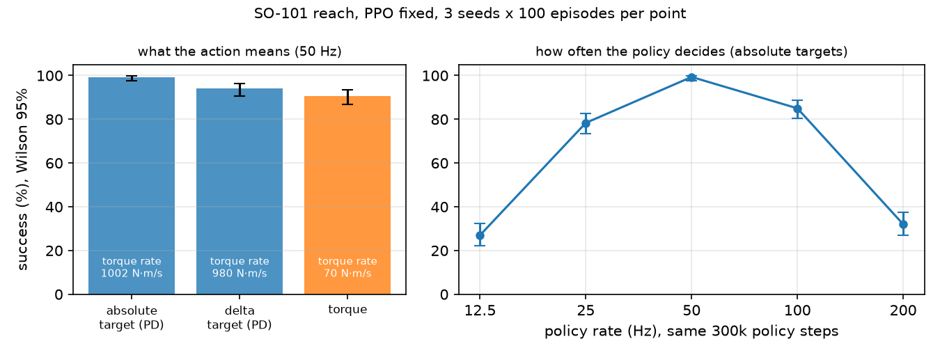
Left: pooled success for the three action interfaces at 50 Hz, 298/300 for absolute targets, 282/300 for delta targets and 272/300 for torque, with torque rates of 1002, 980 and 70 N·m/s. Right: success against policy rate from 12.5 to 200 Hz, an inverted U that peaks at 50 Hz.

There is a sweet spot, and it sits where the Go2 config also sits. Two effects meet. At a fixed number of policy steps, a 200 Hz policy sees only a quarter of the simulated time (and episodes) of a 50 Hz one, and its credit assignment (working out which earlier action caused a later reward) spans 4× more steps for the same horizon. At 12.5 Hz each decision holds for 80 ms, so the policy cannot correct within a motion, and power rises (19.54 W), consistent with the stiff servo chasing larger target jumps. A budget in simulated seconds would give the 200 Hz policy four times more experience (Build it, Step 4); we did not run that variant.

C. Observation content (absolute targets, 50 Hz):

observation	success per seed	pooled	Wilson 95%	final distance (mm)
full: $q$ , $\dot q$ , target − gripper, previous action	100 / 98 / 100	298/300	97.6–99.8%	7.5
without joint velocities	77 / 68 / 80	225/300	69.8–79.6%	14.4
absolute target instead of target − gripper	26 / 40 / 35	101/300	28.6–39.2%	27.7

The relative goal is the single most important input: with the absolute target position the policy has to learn forward kinematics just to know which way to move, and success drops to a third. Dropping velocities costs a quarter of the successes: without $\dot q$ the policy can only infer motion indirectly (from its previous action), so it cannot reliably tell a joint that is arriving from one that is leaving. The Go2 observation likewise includes base and joint velocities.

Break it

Copy the Go2’s action scale, 0.25 rad, onto the arm:

scale	success per seed	pooled	Wilson 95%	final distance (mm)
1.0 rad	100 / 98 / 100	298/300	97.6–99.8%	7.5
0.25 rad	9 / 8 / 4	21/300	4.6–10.5%	62.6

The scripted IK controller, sent through the same clipped interface, reaches 100/100 targets at scale 1.0 and only 27/100 at 0.25. So the failure is not PPO’s: targets are sampled up to 0.6–1.0 rad from $q_0$ , and with $|a| \le 1$ the policy can command at most $q_0 \pm 0.25$ rad, so most targets are outside the action space. The scripted controller’s 27/100 is a reference, not a strict ceiling (the IK is not optimal under clipping). The Go2’s 0.25 works because a trot stays near the default pose; the scale must cover the motion the task needs, and no more, since it also multiplies the exploration noise.

On the real robot

The STS3215 on the SO-101 runs its own position loop, so on the real arm the “absolute target” interface is the native one: the policy writes goal positions over the servo bus. The model’s own comment says its gains are not a one-to-one mapping of the servo gains used on the real arm (so101.xml), so the simulated closed loop is an approximation. Torque mode would need current control, which this lesson did not test on hardware.
For the Go2, the training PD (20 / 0.5) and Unitree’s real-robot stand example (Kp 60, Kd 5, go2_stand_example.py) differ; a policy trained with one set of gains is trained for that closed loop (lesson 12).
Smoothness numbers here are simulation results with an ideal actuator. The real arm’s torque rate was not measured.

Check yourself

Quick check · 2 questions. Click an answer.

1. Absolute joint targets learned best (298/300) but had a torque rate of 1002 N·m/s against 70 N·m/s for raw torques. Where does the jerkiness come from?

The target policy explores with more noise than the torque policy.
The simulated servo is very stiff, so every new 50 Hz target produces a near bang-bang torque step.
The physics timestep of 5 ms is too large for a PD loop.

Why: Section A: with kp = 998.22 and a 2.94 N·m cap, a position error of 3 mrad already saturates the actuator. A PD interface is only as gentle as its gains.

2. With the Go2’s action scale of 0.25 rad, PPO reached 21/300 targets. What does the scripted IK through the same interface (27/100) show?

PPO needed more training steps at the smaller scale.
Smaller scales always give smoother and better policies.
The failure is not PPO’s; most targets lie outside $q_0 \pm 0.25$ rad, the most the policy can command.

Why: Break it. Targets are sampled up to 0.6–1.0 rad from $q_0$ ; at scale 1.0 the same scripted IK reaches 100/100. Size the scale to the motion the task needs.

Easy. In the Go2 config, what joint target does an action of $a = 1$ give for the front-left thigh (default 0.8 rad)? What torque does the PD produce if the joint is still at 0.8 rad and at rest?
Medium. Lower the SO-101 servo gain in the env (e.g. kp = 100, kv scaled to keep the damping ratio) and rerun section A for absolute targets. Predict the direction of torque rate and success before running.
Hard. Repeat section B with a budget in simulated seconds instead of policy steps (e.g. 1500 s of experience for every rate). Does the 200 Hz policy catch up? Report success with Wilson intervals over 3 seeds.

Answers

$q^* = 0.25 \cdot 1 + 0.8 = 1.05$ rad; $\tau = 20 \cdot (1.05 - 0.8) - 0.5 \cdot 0 = 5.0$ N·m.
Open; we did not run it. Expect a lower torque rate (smaller torque per target step); whether success holds depends on whether the softer servo still overcomes gravity at the shoulder.
Open; we did not run it.

Takeaways and sources

Joint targets tracked by a PD loop learned best (298/300); raw torques learned less (272/300) but were an order of magnitude smoother, because the simulated servo is very stiff. Choose the interface and the gains together.
The policy rate has an optimum (50 Hz here: 298/300 vs 96/300 at 200 Hz and 81/300 at 12.5 Hz, same step budget), and $\gamma$ must be retuned when the rate changes.
Put what the task needs in the observation in the frame the policy acts in: target − gripper instead of the absolute target took success from 101/300 to 298/300. Size the action scale to the task: 0.25 rad capped the arm at 21/300.

Next: lesson 35, what the reward asks for and what the agent does with it.

Sources

unitree_rl_gym · go2_config.py, legged_robot.py (_compute_torques, compute_observations), legged_robot_config.py (BSD-3-Clause).
unitree_sdk2_python · go2_stand_example.py.
MuJoCo · XML reference, actuators (position actuator = PD inside the physics step).
MuJoCo Menagerie · robotstudio_so101 (Apache-2.0).
J. Schulman et al., “Proximal Policy Optimization Algorithms”, 2017. arXiv 1707.06347
Code: experiment.py, output.txt; env and PPO from lesson 32 and lesson 33; figure from plot.py.