29 · Distribution shift and DAgger


Part	7 · Learning from demonstration
Run type	CPU · Mac or Colab CPU
Prerequisites	28
Learn first	Bias-Variance Tradeoff
Time	~45 min
Code	`experiments/29-dagger/experiment.py`
Status	✅ done

Act on this lesson

Tick each step when you have done it. Saved in this browser only.

01 · Read The problem and the core idea; answer the questions before you read.
02 · Build it Type the steps yourself, then run uv run python experiments/29-dagger/build.py
03 · Run the experiment Predict first, then run uv run python experiments/29-dagger/experiment.py
04 · Break it Change the one parameter and watch it fail.
05 · Check yourself Quizzes and exercises at the end.

Behavior cloning trains on the expert’s states and runs on its own. DAgger closes that gap by asking the expert what to do in the states the learner actually reaches.

The problem

Lesson 28 ended with a network trained on 50 demonstrations that scores 0/20 without input noise. Nothing is wrong with the regression; the failures happen in closed loop, where the policy’s output moves the robot and the new state is its next input. Ross and Bagnell (2010) named the reason: treating imitation as i.i.d. supervised learning ignores that the learner’s own actions decide which states it sees next, and the regret “grows quadratically in the time horizon of the task”. The gap between the states seen in training and the states met at run time is called distribution shift. This lesson measures it on the SO-101 pick and applies the standard fix, DAgger (Ross, Gordon, Bagnell 2011), with lesson 16’s scripted pick as the expert.

Before you read · 2 questions. Guess first; the lesson tells you why.

1. In the DAgger loop, who chooses the states and who chooses the actions that end up in the dataset?

The expert chooses both; the learner is only retrained.
The learner chooses the states, because it is driving; the expert chooses the actions, the labels.
The learner chooses both, and the expert only scores each rollout.

Why: Core idea, DAgger as code: the learner drives, data.append((s, expert(s))) stores each visited state with the expert’s label, and the policy is retrained on all of it.

2. You learned to drive by watching an instructor who always stays in the middle of the lane. On your first solo drive a small error puts you half a metre to the left. What tends to happen next?

You return to the middle at once, because you saw so many correct drives.
Nothing; a small error stays small.
Your next decision is a guess about a place you never saw, it is a little off, and you drift further; errors compound.

Why: That is distribution shift. In Build it, Step 2, a cloned driver is 0.080 m from the demonstrations in the first 2.5 s and 0.171–0.226 m later, and stays in the lane in 3 of 50 episodes.

Core idea

In plain words

You learn to drive by watching an instructor who always stays in the middle of the lane. You have never seen what to do half a metre to the left, because the instructor was never there. On your first solo drive a small error puts you exactly there, your next decision is a guess, and the car drifts further into places you have never seen. Errors compound. That is distribution shift.

A good instructor fixes this differently: they let you drive, sit next to you, and at every moment say what they would do from where the car actually is. You add those corrections to everything you already know, practise on all of it, and drive again; after a few rounds your notes cover the places where you drift. That is DAgger (Dataset Aggregation). It needs an expert who can answer “what would you do here?” for any state, and it keeps all earlier notes (Break it drops them).

flowchart TD
    D["expert demonstrations"] --> P["dataset<br/>(all rounds kept)"]
    P --> T["train policy"]
    T --> R["policy drives<br/>10 episodes"]
    R --> S["record the states<br/>it actually visits"]
    S --> L["expert labels each state:<br/>what would I do here?"]
    L --> P
    T --> E["evaluate on 20<br/>test positions"]

DAgger as code

def dagger(expert, demos, n_iters, m):
    data = list(demos)                       # (state, action) pairs recorded while the expert drove
    policy = train(data)                     # iteration 0: this is plain behavior cloning
    policies = [policy]
    for i in range(n_iters):
        for _ in range(m):                   # m episodes per iteration (here 10)
            for s in rollout(policy):        # the LEARNER drives, so it picks the states...
                data.append((s, expert(s)))  # ...and the EXPERT picks the action label
        policy = train(data)                 # retrain on everything, not only the newest round
        policies.append(policy)
    return best_on_validation(policies)      # success is not monotonic in the iteration

def drift_deg(q, demo_frames):               # q: 5 joints + jaw of one visited state, in degrees
    return min(max(abs(q - f)) for f in demo_frames)   # 0 = a state the dataset contains

What	Formula
BC cost bound	$J(\hat\pi_{\text{BC}}) \le J(\pi^*) + T^2 \epsilon$
DAgger cost bound	$J(\hat\pi_{\text{DAgger}}) \le J(\pi^*) + u\,T\,\epsilon_N + O(1)$
Shift measure	$\min_j \max_i \lvert q_i - q_i^{(j)}\rvert$

$J$ is the expected cost over an episode of $T$ steps (ours: $T = 150$ policy steps), $\pi^*$ the expert and $\hat\pi$ a learned policy, $\epsilon$ the probability that BC errs on the expert’s states, $\epsilon_N$ the loss of the best policy in hindsight on the states the learned policies visited, $u$ a bound on how much one mistake (followed by the expert) can add to the remaining cost, $q_i$ joint $i$ of a visited state and $q^{(j)}$ demonstration frame $j$ . In words: BC’s extra cost can grow with the square of the episode length, DAgger’s only linearly.

Math details: why BC's error grows with T² and DAgger's with T

Two state distributions. BC minimizes the loss under $d_{\pi^*}$ , the expert’s states; at run time the policy meets $d_{\pi_\theta}$ , its own. Assume a 0-1 loss, a cost per step in [0, 1], and an error probability $\epsilon$ on expert states.

The $T^2$ intuition. One error can move the learner where nothing was trained, and in the worst case it pays the maximum cost from then on. An error can start at any of the $T$ steps (probability about $\epsilon$ each) and can cost up to $T$ , so the extra cost is of order $T \cdot \epsilon T = T^2\epsilon$ . The DAgger paper states this BC bound and its tightness (Ross & Bagnell 2010 give an example that attains it).

The DAgger bound. Algorithm 3.1 runs, at iteration $i$ , the mixture $\pi_i = \beta_i \pi^* + (1-\beta_i)\hat\pi_i$ , labels the visited states with $\pi^*(s)$ , aggregates $\mathcal D \leftarrow \mathcal D \cup \{(s, \pi^*(s))\}$ and trains $\hat\pi_{i+1}$ on all of $\mathcal D$ . Training on the union of all rounds is Follow-The-Leader, a no-regret online learner; that is what turns the $T^2$ into $u\,T\,\epsilon_N$ . The bound holds for some policy among $\hat\pi_{1:N}$ once $N$ is of order $uT$ (Theorems 2.1 and 3.2), which is why the algorithm ends with “Return best $\hat\pi_i$ on validation”.

Our schedule. $\beta_i = \mathbb 1(i = 1)$ : the first data comes from the expert, then the learner drives alone, the paper’s parameter-free version.

Go deeper: Bias-Variance Tradeoff (AIEFS); Ross, Gordon, Bagnell 2011, Algorithm 3.1 and Theorems 2.1, 3.2; Ross & Bagnell 2010; CS 285, lectures 2–3.

The expert as labeler

DAgger needs $\pi^*(s)$ at states the expert never visited. Our expert is the time-indexed state machine of lesson 16, so the label for a learner state at policy step $k$ is the action the scripted pick commands at step $k$ for the cube where it is now. If the learner has pushed the cube more than 1 cm, the expert re-plans for the new position (plans are cached on a 2 mm grid of cube positions). This labeler is exact on schedule and weaker when the learner runs late or early; a human operator has the same limit in a different form.

Build it

The Experiment needs 4.5 minutes of CPU because every round retrains an MLP and rolls out the SO-101 pick. To see the loop itself, you build it on a smaller task that runs in about 3 s: the lane from Core idea. A car drives at 1 m/s along a curved lane ( $y = \sin(x/2)$ , half-width 0.5 m); the state is $(x, y, \psi)$ , the action a steering rate. The expert is a feedback law, so it can label any state. Demonstrations are recorded on a calm day; at test time and during DAgger’s rollouts a gust turns the car by 0.04 rad (standard deviation) per step. The learner is exact on its data and blind elsewhere: the action of the nearest stored state.

The functions are in physai/imitation.py; uv run python experiments/29-dagger/build.py runs the four steps (output in build_output.txt).

Step 1 · The task and the expert

yc, pc = lane(x)                                            # centre line y = sin(x/2) and its heading
u = np.clip(2.0 * (pc - psi) - 3.0 * (y - yc), -2.0, 2.0)   # the expert's steering rate [rad/s]

== Step 1. The task and the expert ==
lane y = sin(x/2), half-width 0.5 m, 1 m/s, 200 steps of 0.05 s; gust std 0.04 rad per step
20 noise-free demonstrations: 4000 states, lateral offset from the centre at most 8.0 cm
expert with gusts: 50/50 episodes stay in the lane

The expert stays in the lane in 50 of 50 gusty episodes, and its 20 demonstrations never leave a band of 8.0 cm around the centre: the instructor always drove in the middle.

Step 2 · Plain BC and the drift measure

The learner and the lesson’s drift measure, $\min_j \max_i |s_i - f_{ji}|$ , both use a k-d tree:

def knn_policy(X, Y):
    """A learner that is exact on its data and blind elsewhere: the action of the nearest stored state."""
    tree = cKDTree(np.atleast_2d(X))
    return lambda S: Y[tree.query(np.atleast_2d(S))[1]]

def nearest_distance(states, frames):
    """Distance of each state to its nearest frame, max-abs over the coordinates: min_j max_i |s_i - f_ji|."""
    d, _ = cKDTree(np.atleast_2d(frames)).query(np.atleast_2d(states), p=np.inf)
    return d

== Step 2. Plain BC: a 1-nearest-neighbour learner on the demonstrations ==
nearest_distance vs brute force on 200 points: max diff 0.0e+00
  demos  success   dist to demos [m] in 0-2.5 / 2.5-5 / 5-7.5 / 7.5-10 s
     20     3/50    0.080  0.171  0.176  0.226
     40     4/50    0.084  0.214  0.140  0.198
     60     4/50    0.071  0.176  0.166  0.166
 expert    50/50    0.021  0.035  0.028  0.032

Cloning the expert gives 3/50, and more demonstrations do not help (4/50 with 40 or 60): every new one again lies in the middle of the lane. The expert’s own gusty episodes stay within 0.021–0.035 m of the demonstrations; the learner’s are 0.080 m away in the first 2.5 s and 0.171–0.226 m later. A gust pushes it off the band, the nearest stored state says “steer as in the middle”, and the next gust adds to the error: the pattern of plain BC’s 22–29° in Experiment A.

Step 3 · DAgger

The whole algorithm is a few lines: the learner drives, the expert labels what the learner saw, everything is kept, and the learner is refit.

def dagger(fit, expert, rollout, X, Y, starts, aggregate=True):
    """DAgger (Ross, Gordon, Bagnell 2011) with beta = 1 only for the initial demonstrations.

    fit(X, Y) -> policy; expert(states) -> action labels; rollout(policy, start) -> states the policy visited.
    starts: one list of start states per iteration. Returns the policies of iterations 0, 1, ..., len(starts).
    """
    policies = [fit(X, Y)]                                   # iteration 0 is plain behavior cloning
    for batch in starts:
        S = np.concatenate([rollout(policies[-1], s0) for s0 in batch])   # the learner drives ...
        A = expert(S)                                                   # ... the expert labels
        X, Y = (np.concatenate([X, S]), np.concatenate([Y, A])) if aggregate else (S, A)
        policies.append(fit(X, Y))
    return policies

== Step 3. DAgger: 10 learner episodes per iteration, labelled by the expert, all data kept ==
 iter  expert-labelled episodes  success   dist to demos [m] per window
    0                        20     3/50    0.080  0.171  0.176  0.226
    1                        30    36/50    0.025  0.053  0.084  0.109
    2                        40    50/50    0.023  0.041  0.036  0.043
    3                        50    50/50    0.022  0.040  0.032  0.038
    4                        60    50/50    0.022  0.038  0.030  0.036

One round lifts success from 3/50 to 36/50, two rounds to 50/50, with the same expert budget that left plain BC at 4/50. The drift falls to the expert’s own level (0.022–0.043 m): the learner’s data now covers the places where it actually drifts. This toy improves monotonically; the SO-101 run did not (50/60 at iteration 3, 45/60 at iteration 4).

Step 4 · Break it: keep only the newest round

== Step 4. Break it: train each iteration only on its newest 10 learner episodes ==
success per iteration 0..4: 3/50 2/50 0/50 40/50 50/50

Without aggregation iterations 1 and 2 get worse (2/50, then 0/50), as in the Experiment. Unlike on the arm, iterations 3 and 4 recover (40/50, 50/50): a nearest-neighbour learner is exact on whatever it was given, so once one round stays near the lane, the next round’s data is good data. The MLP on the pick had no such luck (0/20 in every iteration). The guarantee in Math details is for the aggregated dataset; without it the outcome depends on the learner and the task.

What you keep

physai.imitation now also has nearest_distance, knn_policy and dagger. dagger takes any fit, expert and rollout, so the same loop drives the MLP and the scripted labeler of the Experiment. tests/test_29_dagger.py checks the drift measure against brute force and that DAgger labels and aggregates the learner’s states; run uv run pytest tests/test_29_dagger.py.

Use it

In simulation you write the loop yourself around your trainer, as in Step 3, with a scripted or model-based expert called on every state the learner visits (the Experiment ran the scripted expert 1327 times). On the real SO-101 the expert is you, and LeRobot ships the loop as a rollout strategy (Human-In-the-Loop Data Collection):

lerobot-rollout --strategy.type=dagger --policy.path=<trained policy> \
    --robot.type=so_follower --teleop.type=so_leader \
    --dataset.repo_id=<user>/<hil dataset> --strategy.num_episodes=50 ...

The policy drives; you pause it when failure looks imminent, take over with the leader arm, recover and correct, and hand control back. Then you fine-tune on the demonstrations and the new data merged, and repeat. The prerequisite is a leader arm with active motors (it must move itself to mirror the follower when you pause); so_leader is on the docs’ list. The pieces map like this:

DAgger piece	Step 3 / the Experiment	LeRobot `--strategy.type=dagger`
who picks the states	the learner, in simulation	the policy, on the robot
expert labels	every visited state, scripted	only where the operator intervenes (HG-DAgger gating)
aggregation	all rounds concatenated	fine-tune on demonstrations + HIL data merged
next round	refit, roll out 10 new episodes	deploy the fine-tuned policy, collect again

Three traps:

Label timing. A time-indexed expert gives the wrong label when the learner is late or early (The expert as labeler, above); a human corrects with a reaction-time delay.
Overwriting the dataset. Training only on the newest round is the Break it; keep every round.
Picking the last iteration. Success is not monotonic (45/60 after 50/60 in the Experiment); evaluate every round on the same held-out positions and keep the best.

Check after building · 2 questions.

1. In Build it, Step 2, plain BC stays in the lane in 3/50 episodes with 20 demonstrations and 4/50 with 40 or 60. Why do more demonstrations barely help?

Every new demonstration again lies in the middle of the lane, so none of them shows what to do where the learner drifts.
The nearest-neighbour learner can store only 20 demonstrations.
The gusts are stronger when there are more demonstrations.

Why: The 20 demonstrations never leave a band of 8.0 cm around the centre. DAgger with the same budget reaches 36/50 after one round and 50/50 after two (Step 3).

2. With lerobot-rollout --strategy.type=dagger on the SO-101, which states get an expert label?

Every state the policy visits, as in Step 3.
Only the stretches where the operator pauses the policy and takes over with the leader arm (HG-DAgger gating).
None; the strategy only records the policy’s own actions.

Why: Use it, the table. Both autonomous and human segments are recorded, and the policy is fine-tuned on demonstrations plus the new data merged.

Experiment

Setup: lesson 28’s features (state + clock) and MLP, trained without input noise (“plain BC”), 20 demonstrations, the same 20 test positions, 3 seeds. DAgger adds 10 learner episodes per iteration at fresh cube positions, 4 iterations; the baseline is plain BC on the same number of scripted demonstrations. Full script: experiments/29-dagger/experiment.py, output: output.txt. MuJoCo 3.17.0, NumPy 2.5.4, PyTorch 2.14.1 (CPU), Apple Silicon Mac (Apple M5), deterministic, about 4.5 min of CPU (approximate; wall time was several times longer on a heavily loaded machine).

for it in range(1, ITERS + 1):
    for xy in L26.sample_positions(ROLLOUTS, seed=1000 * seed + it):
        _, x, y, _ = run_episode(scene, labeler, pol, xy, label=True)   # learner drives
        nx += x; ny += y                                                # expert labels
    X, Y = np.concatenate([X, nx]), np.concatenate([Y, ny])             # aggregate
    pol = L28.train_mlp(X, Y, seed=seed)                                # retrain on all

Predict: plain BC fails at 20 demonstrations. Does it recover with 40 or 60 demonstrations? Does DAgger with the same number of expert-labelled episodes?

B. DAgger vs plain BC. “Pooled” sums the three seeds; “dist” is the mean distance of visited arm states to the nearest frame of the 20 initial demonstrations (also for the BC rows trained on 40 and 60).

Iteration	expert-labelled episodes	DAgger, seeds 0/1/2	pooled	Wilson 95%	dist [deg]	plain BC, seeds 0/1/2	pooled	dist [deg]
0	20	0/0/0	0/60	[0.00, 0.06]	29.35	0/0/0	0/60	29.35
1	30	3/18/5	26/60	[0.32, 0.56]	15.79	–	–	–
2	40	19/11/12	42/60	[0.57, 0.80]	12.59	0/0/0	0/60	26.75
3	50	19/16/15	50/60	[0.72, 0.91]	6.09	–	–	–
4	60	15/15/15	45/60	[0.63, 0.84]	7.50	0/0/0	0/60	24.76

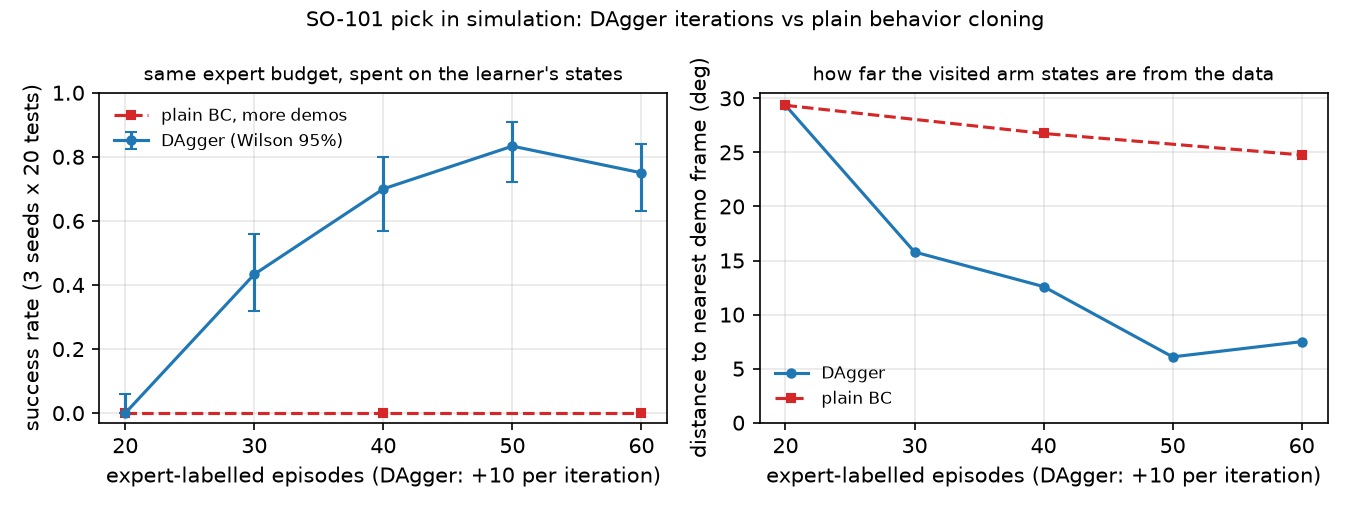
Two panels against the number of expert-labelled episodes (20 to 60). Left: DAgger's pooled success rises from 0 to 50 of 60 at 50 episodes and falls slightly to 45 of 60 at 60, while plain BC stays at 0 of 60. Right: DAgger's mean distance to the demonstrations falls from 29 to about 6 to 8 degrees, plain BC's only to about 25 degrees.

(Plain BC was retrained only at 40 and 60 episodes, to save CPU.) Tripling the demonstrations does nothing for plain BC: 0/60 at 20, 40 and 60 episodes, its states 25–29° from the initial demonstrations. The same expert budget spent by DAgger on the learner’s own states lifts success to 50/60 after three iterations, and the distance falls to about 6°. Iteration 4 is lower (45/60, overlapping intervals): DAgger does not improve monotonically, hence “Return best $\hat\pi_i$ on validation”. The labels are not free: the scripted expert ran 1327 times; at most 180 of those are fresh start positions (20 test + 160 collection episodes), the rest re-plans after the learner pushed the cube more than 1 cm.

A. Where the learner goes. Mean distance to the nearest demonstration frame [deg] per time window, seed 0:

Policy	0–1 s	1–2 s	2–3 s	3–4.5 s	4.5–6 s	success	mean max deviation from expert trajectory [deg]
plain BC, 20 demos	22.44	29.05	28.96	28.94	28.87	0/20	62.6
BC + input noise (lesson 28), 20 demos	1.80	4.52	4.94	4.46	3.85	20/20	10.7
DAgger after 4 iterations	2.27	4.97	7.38	15.10	15.95	15/20	19.0

Plain BC is 22° from every demonstrated arm configuration in the first second and about 29° after that: the compounding happens within the first 25 policy steps. Both fixes stay under 5° during the approach. DAgger’s states drift later (15° after 3 s), but its dataset contains those states with expert labels, so far from the demonstrations is not far from the training data. Lesson 28’s noise-trained policy is the best here, 20/20 with no extra expert queries: input noise is a cheap, local stand-in for on-policy data, enough while the learner’s errors stay small.

Break it

Aggregation is the “Agg” in DAgger. Train each iteration only on its newest 10 learner episodes (dropping the demonstrations and earlier rounds), seed 0:

Iteration	0	1	2	3	4
success without aggregation	0/20	0/20	0/20	0/20	0/20
success with aggregation	0/20	3/20	19/20	19/20	15/20

Without aggregation every iteration fails. Our reading: each new dataset contains only the states the previous, failing policy visited, mostly after its mistakes. A policy trained on those alone has never seen the approach done right, so it fails in a new way, and the next dataset covers only that failure. The paper’s guarantee rests on training on the union of all rounds (Follow-The-Leader); the demonstrations anchor the policy on the expert’s states, the learner’s states teach recovery. (Build it’s lane toy shows that a different learner can recover without it.)

On the real robot

LeRobot runs the loop with a human expert (lerobot-rollout --strategy.type=dagger, see Use it). The docs name DAgger, HG-DAgger and RaC as the ideas behind it.
What changes with a human labeler. In human-in-the-loop (HIL) collection the human intervenes only when failure looks imminent (the HG-DAgger gating), so the labels cover the states where the learner was about to fail rather than every visited state as in our loop. Labels are also noisier and slower than a script’s.
Not yet measured on the real arm. Procedure: train a policy on 20 teleoperated episodes, evaluate it on 20 marked positions (lesson 25), run 2–3 rounds of --strategy.type=dagger with 10 episodes each, fine-tune, and re-evaluate on the same positions; report k/20 and Wilson intervals after each round, next to a policy trained on the same number of plain teleoperated episodes.

Check yourself

Quick check · 2 questions. Click an answer.

1. Plain BC scores 0/60 with 20, 40 and 60 expert-labelled episodes. What does DAgger do with the same expert budget?

Also 0/60: more expert labels cannot help a regression.
60/60 at every iteration after the first.
50/60 after three iterations, with visited states about 6° from the demonstrations instead of about 25°.

Why: Part B table: 26/60, 42/60, 50/60, 45/60 for iterations 1–4, distance 6.09° at iteration 3 against 24.76° for plain BC at 60 episodes; success is not monotonic, hence “return the best policy on validation”.

2. Break it trains each iteration only on its newest 10 learner episodes, without the demonstrations or earlier rounds. What happens?

Every iteration scores 0/20: each new dataset covers only the states the previous, failing policy visited, mostly after its mistakes.
It learns faster, because old data no longer dilutes the new labels.
Nothing changes, because the expert’s labels are the same.

Why: Break it table: 0/20 at every iteration without aggregation, against 3, 19, 19 and 15/20 with it; the paper’s guarantee rests on training on the union of all rounds.

Easy. In the DAgger loop above, who chooses the states and who chooses the actions that end up in the dataset?
Medium. Lesson 28’s input noise also lifted plain BC to 20/20 at 20 demonstrations. Explain why it works and why it is not a general replacement for DAgger.
Hard. Add a mid-episode perturbation to evaluation (move the cube 3 cm at t = 1.6 s) and repeat the DAgger loop with the same perturbation during collection. Predict the gap to plain BC, then measure it.

Answers

The learner chooses the states (it is driving); the expert chooses the actions (the labels).
Noise trains the policy on states near the demonstrations with the expert’s action from the nearby demonstration state, which is a good label only when the correct action changes little across that neighbourhood. DAgger labels the states the learner actually reaches, however far they are, with the expert’s action for that state.
Not computed here; run it.

Takeaways and sources

In simulation, plain BC (no input noise) scored 0/60 at 20, 40 and 60 demonstrations; DAgger with the same expert budget reached 50/60 after three iterations.
The shift is measurable: plain BC’s arm states were 22–29° from every demonstrated configuration, DAgger’s 6–8° (mean) after three to four iterations.
Aggregate: retraining only on the newest learner data scored 0/20 at every iteration. Here lesson 28’s input noise (20/20, no expert queries) was the cheaper fix; DAgger is the general one.

Next: lesson 30 · Multimodal actions: diffusion and flow policies.

Sources:

S. Ross, G. J. Gordon, J. A. Bagnell, “A Reduction of Imitation Learning and Structured Prediction to No-Regret Online Learning”, AISTATS 2011 (Algorithm 3.1, Theorems 2.1 and 3.2).
S. Ross, J. A. Bagnell, “Efficient Reductions for Imitation Learning”, AISTATS 2010.
LeRobot, Human-In-the-Loop Data Collection and Imitation learning on real-world robots (read 2026-10-27).
UC Berkeley CS 285 Deep Reinforcement Learning, lectures 2–3 “Behavioral Cloning”.
All measured numbers: experiments/29-dagger/output.txt.