28 · Behavior cloning


Part	7 · Learning from demonstration
Run type	CPU · Mac or Colab CPU
Prerequisites	27
Learn first	Multi-Layer Networks and Forward Pass · Loss Functions · Introduction to PyTorch
Time	~60 min
Code	`experiments/28-behavior-cloning/experiment.py`
Status	✅ done

Act on this lesson

Tick each step when you have done it. Saved in this browser only.

01 · Read The problem and the core idea; answer the questions before you read.
02 · Build it Type the steps yourself, then run uv run python experiments/28-behavior-cloning/build.py
03 · Run the experiment Predict first, then run uv run python experiments/28-behavior-cloning/experiment.py
04 · Break it Change the one parameter and watch it fail.
05 · Check yourself Quizzes and exercises at the end.

Behavior cloning is supervised regression from states to the expert’s actions. Its loss is measured on frames, its success only in closed loop, and the two can disagree.

The problem

Lessons 26–27 left us 120 scripted demonstrations and a clean dataset. The simplest way to turn them into a policy is behavior cloning (BC): fit $\pi_\theta(o) \approx a$ by regression, the recipe behind ALVINN, which learned to steer a vehicle from camera and laser range images (Pomerleau, NIPS 1988). The questions a robotics engineer has to answer before trusting it are concrete. How many demonstrations does an SO-101 pick need? Does a lower validation loss mean more successful picks? And what makes a network that fits the data almost perfectly drop the cube anyway?

Before you read · 2 questions. Guess first; the lesson tells you why.

1. In a recorded game, one screen is followed by “wait” in most frames and by “jump” in a few, because the player waited, then jumped. What does a regression from screen to key learn for that screen?

Exactly when to jump, because the network sees enough frames.
Nothing; regression cannot be trained on repeated inputs.
Something close to the average action, so mostly “wait”; the screen alone does not say when the decision comes.

Why: For a fixed input, MSE learns the mean of the actions seen with it (Math details). On the arm, removing the clock left 16 of 20 episodes with the jaws never closing (Break it).

2. Your cloned policy has a tiny error on recorded frames. What tells you whether it actually picks the cube?

Running it in closed loop, where it feeds itself its own states, and applying the physical success test.
The error on frames; a smaller error always means more successful picks.
The training loss on the last batch.

Why: The open-loop RMSE averages over demonstration frames; success depends on a few decisive states and on states the expert never visited. Experiment A shows the two disagreeing.

Core idea

In plain words

Suppose you want a bot that plays a video game. You record a good player: at every frame, the screen and the key they press, and train an ordinary supervised model on those pairs: screen in, key out. That is behavior cloning: no reward, no trial and error, only recorded pairs. For our robot the “screen” is the joint angles plus the cube position, and the “keypress” is the next set of joint targets.

Two things go wrong. The bot never plays exactly like the player, so after a few frames it sees screens the player never produced, where it has no data, and each small mistake pushes it further off. And sometimes the screen alone does not say what to do: the player waited, then pressed jump, and the screens just before and after that decision look the same. Finally, the score you watch during training (error on recorded frames) is not the score that matters (is the cube lifted when the bot plays alone); this lesson measures both.

Training on frames, running in a loop

flowchart TD
    D["demos: (state, expert action) pairs"] --> T["fit an MLP by regression<br/>(MSE on frames)"]
    T --> P["policy"]
    P --> A["action: 6 joint targets"]
    A --> S["simulate 40 ms"]
    S --> O["new state: the policy's own,<br/>not the expert's"]
    O --> P
    S --> C["after 6 s:<br/>physical success test"]

Behavior cloning, as code

# Training: ordinary supervised regression on (observation, expert action) pairs
for step in range(4000):
    x, a = sample_batch(demos, 256)           # x: 9 state values + clock t, a: expert action (6)
    x_in = x + noise_like(x)                  # 0.02 rad on joints and jaw, 1 mm on the cube, 0 on t
    pred = policy(normalize(x_in))            # MLP 2 x 256, MEAN_STD from lesson 27
    loss = ((pred - normalize_a(a)) ** 2).mean()  # MSE against the clean expert targets
    loss.backward(); opt.step(); opt.zero_grad()

# Run time: the policy feeds itself (closed loop)
for k in range(150):                          # 6 s at 25 Hz
    x = concat(scene.obs(), min(k / 25, 4.52))   # clock clipped to the last demo timestamp
    a = unnormalize_a(policy(normalize(x)))
    scene.apply(a); scene.step(20)            # hold 40 ms

Quantity	Formula
BC objective	$\theta^* = \arg\min_\theta \; \mathbb E_{(o,a) \sim \mathcal D}\, \big\\| \pi_\theta(o) - a \big\\|^2$
with input noise	$\mathbb E_{(o,a) \sim \mathcal D,\ \epsilon}\, \big\\| \pi_\theta(o + \epsilon) - a \big\\|^2$
open-loop RMSE	$\sqrt{\operatorname{mean}\big(\pi_\theta(o) - a\big)^2}$ over held-out demo frames
closed-loop success	$k/n$ from the physical test of lesson 25

Here $\theta$ are the network weights, $\pi_\theta$ the policy, $\mathcal D = \{(o_t, a_t)\}$ the demonstrations of the expert $\pi^*$ , $o$ an observation (9 state values plus the clock), $a$ the expert’s action (6 joint targets) and $\epsilon$ Gaussian noise (0.02 rad per joint, 1 mm on the cube). The catch is the training distribution: $o$ comes from the states the expert visits, while at run time the policy feeds itself its own states. Lesson 29 deals with that gap.

Our policy

Part	Choice
input	5 arm joints, jaw, cube xyz (9) + episode clock $t$ (clipped to 4.52 s, the last demo timestamp)
output	next 6 joint targets [rad], held for 40 ms (20 physics steps)
network	MLP 2 × 256 ReLU, MEAN_STD normalization from lesson 27
training	Adam, lr 1e-3, batch 256, 4000 steps, MSE
augmentation	Gaussian noise on the inputs of each batch: 0.02 rad on joints, 1 mm on the cube; targets unchanged

Why the clock and the noise. The scripted expert is a state machine with timed segments. At the bottom of the descent, “jaws open, at the cube” looks the same just before and just after the expert decides to close; the clock tells them apart. The demonstrations are noise-free curves in a 10-D input space, and off those curves the network’s output is unconstrained. Training on slightly perturbed inputs with the expert’s clean actions maps nearby states onto the expert’s targets, and because the targets are absolute joint positions, the same target pulls a displaced arm back. Both are design choices of this lesson, not part of BC; Break it measures them (50 demos, seed 0): 20/20 with both, 0/20 without noise, 4/20 without the clock.

Closed-loop evaluation. Every 40 ms the policy reads the simulated state and outputs joint targets for the SO-101 position servos; after 6 s the physical test of lesson 25 decides. Each configuration runs with 3 training seeds on the same 20 test positions (seed 28, never used for training); we report each seed’s k/20 and the pooled k/60 with a Wilson interval.

Math details: what MSE regression learns, and why the loop changes things

MSE learns the average action. For a fixed input $o$ , the value $\hat a$ that minimizes $\mathbb E\,\|\hat a - a\|^2$ over the actions seen with that input is their mean, $\mathbb E[a \mid o]$ . If one state is followed by “keep open” in most frames and by “start closing” in a few, the regression outputs something close to “keep open”. Adding the clock makes those frames different inputs, so each gets its own mean.

Training and run-time inputs differ. Training draws $o$ from the expert’s state distribution. At run time $o_{t+1}$ is produced by the simulator from $o_t$ and the policy’s own action $\pi_\theta(o_t)$ , so any action error moves the next input. If the network is accurate only on the expert’s states, a small error takes it to a state where it is less accurate, and the errors compound over the 150 steps of an episode.

Why input noise helps here. Minimizing $\mathbb E\,\|\pi_\theta(o + \epsilon) - a\|^2$ asks the network to output the expert’s action for every state in a small neighbourhood of the demonstrations, not just on the curves themselves. Because $a$ is an absolute joint target, outputting it from a slightly displaced state commands a move back toward the demonstrated path. This is a property of our action space; with velocity or delta actions the argument does not carry over directly.

Go deeper: Multi-Layer Networks and Forward Pass, Loss Functions, Introduction to PyTorch; Pomerleau (1988) and UC Berkeley CS 285, lectures 2–3, in the sources below.

Build it

You will now write behavior cloning yourself: the normalization, the network’s forward pass, the training loop and the closed-loop rollout, each checked before you move on. The data is lesson 26’s demonstrations and the features are this lesson’s (state plus clock), loaded from the Experiment script, so both tell one story. This is a smaller run than the Experiment: one training seed and 20 demonstrations, about 6 s on a CPU.

Type the steps into a file of your own instead of copying them. The finished functions are in physai/imitation.py; uv run python experiments/28-behavior-cloning/build.py runs all four steps (output in build_output.txt).

Step 1 · Normalize

Joint angles are around 1 rad, cube coordinates a few centimetres, the clock up to 4.52 s. Each input is shifted by its mean and divided by its standard deviation (MEAN_STD, lesson 27), and the actions get the same treatment:

def fit_mean_std(x, eps=1e-6):
    """MEAN_STD normalization statistics per feature (lesson 27): shift and scale."""
    x = np.asarray(x, np.float32)
    return x.mean(0), x.std(0) + eps

The check compares the statistics with the ones lesson 27’s trainer computes inside train_mlp:

== Step 1. Normalization statistics, 20 demonstrations ==
2280 frames, 10 inputs (5 joints, jaw, cube xyz, clock), 6 actions
mean   -0.010  -0.256   0.221   1.375   1.623   0.731   0.221   0.014   0.036   2.260
std     0.204   0.508   0.387   0.202   0.204   0.505   0.035   0.045   0.032   1.316
max |ours - lesson 27| = 0.0e+00

The cube’s x has a standard deviation of 0.035 m, its z of 0.032 m; without normalization these inputs would be about 6 to 16 times smaller than the joints and the network would barely see them.

Step 2 · The forward pass

The policy is two ReLU layers of 256 and a linear output. In NumPy that is a loop over the layers:

def mlp_forward(layers, x):
    """ReLU MLP in NumPy: layers = [(W, b), ...] with W of shape (out, in); no activation on the last layer."""
    h = np.asarray(x, np.float64)
    for i, (W, b) in enumerate(layers):
        h = h @ W.T + b
        if i < len(layers) - 1:
            h = np.maximum(h, 0.0)
    return h

Copy the weights of a randomly initialized torch.nn.Sequential into the list and compare outputs:

== Step 2. Forward pass: NumPy vs torch.nn.Sequential (float64, random weights) ==
500 inputs: max |mlp_forward - torch| = 4.4e-16

The difference is rounding (4.4e-16). Running the policy in NumPy keeps PyTorch out of the 25 Hz control loop.

Step 3 · The training loop

Training is ordinary regression on random batches of frames. The one robotics-specific line adds Gaussian noise to the inputs and keeps the expert’s clean action as the label:

def train_bc(X, Y, hidden=256, steps=4000, batch=256, lr=1e-3, seed=0, obs_noise=None):
    """Behavior cloning: MSE regression from observations X to expert actions Y with a 2 x hidden ReLU MLP (Adam).

    Inputs and targets are MEAN_STD-normalized; obs_noise (raw units, one std per input feature) is added to the
    inputs of every batch, the targets stay clean. Returns (layers, x_stats, y_stats) for `bc_policy`.
    """
    import torch
    import torch.nn as nn
    torch.manual_seed(seed)
    g = torch.Generator().manual_seed(seed)
    X, Y = np.asarray(X, np.float32), np.asarray(Y, np.float32)
    (xs, xk), (ys, yk) = fit_mean_std(X), fit_mean_std(Y)
    xt, yt = torch.tensor(X), torch.tensor((Y - ys) / yk, dtype=torch.float32)
    XS, XK = torch.tensor(xs, dtype=torch.float32), torch.tensor(xk, dtype=torch.float32)
    NZ = None if obs_noise is None else torch.tensor(obs_noise, dtype=torch.float32)
    net = nn.Sequential(nn.Linear(X.shape[1], hidden), nn.ReLU(), nn.Linear(hidden, hidden), nn.ReLU(),
                        nn.Linear(hidden, Y.shape[1]))
    opt = torch.optim.Adam(net.parameters(), lr)
    for _ in range(steps):
        idx = torch.randint(0, len(xt), (batch,), generator=g)        # a random batch of frames
        x = xt[idx]
        if NZ is not None:
            x = x + torch.randn(x.shape, generator=g) * NZ           # perturb the input, keep the label
        loss = ((net((x - XS) / XK) - yt[idx]) ** 2).mean()         # MSE in normalized action units
        opt.zero_grad()
        loss.backward()
        opt.step()
    layers = [(m.weight.detach().double().numpy(), m.bias.detach().double().numpy()) for m in net if isinstance(m, nn.Linear)]
    return layers, (xs.astype(np.float64), xk.astype(np.float64)), (ys.astype(np.float64), yk.astype(np.float64))

def bc_policy(layers, x_stats, y_stats):
    """The trained network as a function raw observation(s) -> raw action(s): normalize, forward, unnormalize."""
    (xs, xk), (ys, yk) = x_stats, y_stats
    return lambda x: mlp_forward(layers, (np.atleast_2d(x) - xs) / xk) * yk + ys

The first check trains 200 steps with your function and with lesson 27’s train_mlp (same seed, same noise) and compares the weights. The second trains the full 4000 steps and measures the open-loop error on the 20 held-out episodes:

== Step 3. Training: ours vs lesson 27's train_mlp, then the full run ==
200 steps, same seed: max |weights ours - lesson 27| = 0.0e+00
4000 steps, seed 0: open-loop RMSE on episodes 100-119 = 0.883 deg (predicting the mean action: 23.753 deg)

Identical weights mean your loop is the Experiment’s loop. The open-loop RMSE of seed 0, 0.883°, is close to the Experiment’s 0.945°, which is the mean of three seeds; predicting the mean action everywhere would give 23.753°.

Step 4 · Close the loop

Now the policy drives: every 40 ms it reads the simulated state, the servos chase its six joint targets for 20 physics steps, and after 6 s the physical test of lesson 25 decides.

pi = bc_policy(layers, x_stats, y_stats)
outs = [exp.rollout(scene, lambda o, t: pi(exp.features(o, t))[0], xy) for xy in exp.TEST_XY]

== Step 4. Closed loop: 20 test positions (seed 28), 6 s each ==
success 20/20, Wilson 95% [0.84, 1.00]; outcomes: held 20

20/20, the Experiment’s seed-0 entry at 20 demonstrations. A Wilson interval of [0.84, 1.00] from one seed and 20 positions is still wide; that is why the Experiment pools three seeds.

What you keep

physai.imitation now has fit_mean_std, mlp_forward, train_bc and bc_policy. Lesson 29 adds DAgger to the same module, and lesson 30’s flow-matching sampler replaces the regression when the demonstrations disagree. tests/test_28_behavior_cloning.py pins them to NumPy and to lesson 27’s trainer; run uv run pytest tests/test_28_behavior_cloning.py after you change anything.

Use it

The library way to train a BC-family policy on a real arm is LeRobot. A policy class reads a LeRobotDataset, normalizes with the dataset’s meta/stats.json, and is trained and evaluated from the command line (il_robots):

lerobot-train --dataset.repo_id=<user>/<dataset> --policy.type=act   # or diffusion, ...
lerobot-rollout ...                                                  # evaluate on the robot

The order is the one you built: statistics first, then the network, then closed-loop evaluation. What changes between tools is where each piece lives:

Piece	This lesson / physai	LeRobot ACT	PyTorch by hand
normalization	`fit_mean_std`, MEAN_STD	`normalization_mapping`, MEAN_STD for state, action and images by default	your own `(x - mean) / std`
policy output	the next 6 joint targets	a chunk of `chunk_size` actions (default 100)	whatever the last layer outputs
run time	`bc_policy` in NumPy, 25 Hz	`select_action`, which queues `n_action_steps` actions	`net.eval()` and `torch.no_grad()`

Source: LeRobot’s configuration_act.py and modeling_act.py.

Three traps:

Statistics from the wrong split. Compute mean and std on the training episodes only and ship them with the weights; a policy run with different statistics sees shifted inputs and fails without an error.
Time-indexed demonstrations. A state-only policy cannot tell “before” from “after” a decision the state does not show (Break it: 4/20 without the clock). Check whether your expert has hidden phases before you blame the network.
A low validation loss is not a success rate. Step 3’s 0.883° says little about Step 4; only the closed-loop test does (Experiment A: the RMSE keeps falling while success does not).

Check after building · 2 questions.

1. In Build it, Step 3, train_bc adds torch.randn(...) * NZ to each batch. What does that line do, and what stays unchanged?

It adds noise to the expert’s action labels so the policy explores.
It perturbs the inputs (0.02 rad on joints and jaw, 1 mm on the cube, 0 on the clock) and keeps the expert’s clean action as the label.
It replaces normalization, so fit_mean_std is no longer needed.

Why: Nearby states are mapped onto the expert’s target, and an absolute joint target pulls a displaced arm back. With the same seed and noise, 200 steps of train_bc give weights identical to lesson 27’s train_mlp (difference 0.0e+00).

2. Step 4 gives 20/20 with one training seed, Wilson 95% [0.84, 1.00]. Why does the Experiment still pool three seeds?

Because 20/20 is impossible and must be a bug.
Because the Wilson interval only works for 60 trials.
Because 20 trials from one trained policy leave a wide interval, and another seed can fail where this one succeeded (the 100-demo row has 18, 18 and 19 of 20).

Why: Seed-to-seed variation is part of the result. Pooling gives 60/60 at 20 demos with [0.94, 1.00], still with the caveat that the three seeds share the same 20 test positions.

Experiment

Full script: experiments/28-behavior-cloning/experiment.py, output: output.txt. MuJoCo 3.17.0, NumPy 2.5.4, PyTorch 2.14.1 (CPU, 1 thread), Apple Silicon Mac (Apple M5), deterministic, about 1 min of CPU.

def train_policy(obs, act, t, seed=0, sigma_rad=0.02, clock=True, steps=4000):
    X = features(obs, t, clock)                        # [joints, jaw, cube xyz, t]
    return train_mlp(X, act, steps=steps, seed=seed,   # MEAN_STD inside
                     obs_noise=noise_vector(sigma_rad, clock))

for k in range(150):                                   # 6 s at 25 Hz
    a = policy(scene.obs(), k / 25)
    scene.apply(a); scene.step(20)                     # hold 40 ms
success = scene.success()                              # lifted >= 4 cm, both jaws touching

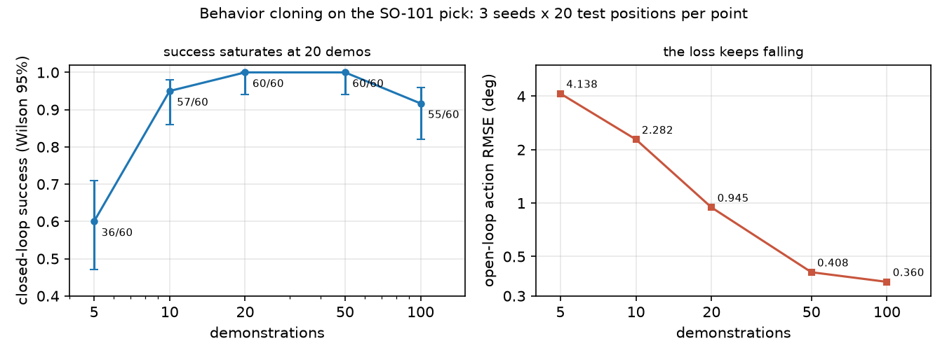
Predict: how many demonstrations until 20/20, and does the open-loop error predict the success rate?

A. Number of demonstrations.

Demos	frames	seeds 0 / 1 / 2	pooled	Wilson 95%	open-loop RMSE [deg]	failed test positions (×seeds)
5	570	12 / 11 / 13	36/60	[0.47, 0.71]	4.138	9 positions, all “closed, cube on floor”
10	1140	19 / 19 / 19	57/60	[0.86, 0.98]	2.282	#4 (16.6, −6.6) cm ×3
20	2280	20 / 20 / 20	60/60	[0.94, 1.00]	0.945	–
50	5700	20 / 20 / 20	60/60	[0.94, 1.00]	0.408	–
100	11400	18 / 18 / 19	55/60	[0.82, 0.96]	0.360	#19 (16.2, 2.7) cm ×3, #3, #7 ×1

Open-loop RMSE is measured on the 20 unseen demo episodes (100–119). Three things stand out:

Success saturates long before the loss does. 60/60 at 20 demos; from 20 to 100 demos the RMSE still falls from 0.945° to 0.360°.
More data was not monotonically better. At 100 demos the pooled rate drops to 55/60; the 95% intervals of 50 and 100 demos barely overlap ([0.94, 1.00] vs [0.82, 0.96]). A two-sided Fisher test on 60/60 vs 55/60 gives p = 0.057, and it treats the 60 rollouts as independent, which they are not (same demos, same 20 positions). The failures concentrate on test position #19, at x = 16.2 cm, the near edge of the demonstrated area, where all three seeds fail. The drop is not statistically established, but not dismissible noise either. With a fixed 4000 training steps, 100 demos means fewer passes over each episode; we did not isolate the cause.
Failures are physical, not numerical. With 5 demos the arm closes the jaws but the cube stays on the floor (24 of 24 failures): the aim is off by more than the grasp tolerance of lesson 26.

Left: pooled closed-loop success with Wilson 95% intervals versus the number of demonstrations: 36/60 at 5, 57/60 at 10, 60/60 at 20 and 50, 55/60 at 100. Right: open-loop action RMSE on a log scale keeps falling, from 4.138 degrees at 5 demos to 0.360 at 100.

Break it

Two knobs, 50 demonstrations, seed 0 (noise 0 turns off the 1 mm cube noise too; the other rows keep it):

Input noise [rad]	clock	success	Wilson 95%	failures
0	yes	0/20	[0.00, 0.16]	closed, cube on floor 20
0.005	yes	0/20	[0.00, 0.16]	never closed 20
0.01	yes	7/20	[0.18, 0.57]	closed, cube on floor 6; lifted, not held 7
0.02	yes	20/20	[0.84, 1.00]	–
0.04	yes	20/20	[0.84, 1.00]	–
0.02	no	4/20	[0.08, 0.42]	never closed 16

Without input noise the policy fits the demonstrations and fails every test: 0/20 at 0 and at 0.005 rad. Our reading, consistent with the drift measured in lesson 29: each 40 ms step adds a small error, the next input lies slightly off the narrow tube of demonstrated states, the output there is extrapolated, and the errors compound. Remove the clock instead and 16 of 20 episodes end with the jaws never closing: “arm at the cube, jaws open” is followed by “keep open” in most frames and by “start closing” in a few, so a state-only regression averages toward “keep open” (our reading, as in Math details).

On the real robot

LeRobot trains BC-family policies with lerobot-train --policy.type=act (and others) on a recorded dataset, and evaluates them with lerobot-rollout (il_robots). Its policies take camera images; our state-only policy reads the cube position from the simulator, which a real arm must estimate from cameras (Part 5).
Not yet measured on the real arm. Procedure: record 10, 20 and 50 teleoperated episodes over the same cube area, train one policy per size, evaluate each on the same 20 marked positions as in lesson 25, and report k/20 with Wilson intervals and failure types. Expect a different curve: human demonstrations are noisier and less consistent than scripted ones, which acts partly like the input noise above and partly like label noise.
The input-noise trick has a hardware analogue: demonstrations that already contain small corrections. That is what DAgger (lesson 29) collects deliberately.

Check yourself

Quick check · 2 questions. Click an answer.

1. From 20 to 100 demonstrations the open-loop RMSE falls from 0.945° to 0.360°. What does closed-loop success do?

It rises steadily and reaches its best value at 100 demos.
It is 60/60 at 20 and 50 demos and 55/60 at 100: a lower loss did not mean more picks.
It falls to 0/60, because the network overfits.

Why: Part A table; a Fisher test on 60/60 vs 55/60 gives p = 0.057, so the drop is not statistically established, but success clearly stopped following the loss.

2. Trained without input noise on 50 demonstrations, the policy scores 0/20. What is the lesson’s reading?

The learner leaves the narrow tube of demonstrated states, its output there is extrapolated, and the errors compound step after step.
Noise-free data is too easy, so the network cannot fit it.
Without noise the network ignores the clock input.

Why: Break it table: 0/20 at 0 and 0.005 rad, 7/20 at 0.01 rad, 20/20 at 0.02 and 0.04 rad; lesson 29 measures the drift directly.

Easy. With 5 demos, which failure type dominates, and what does it say about the policy’s aim?
Medium. RMSE at 50 demos is 0.408°, at 100 it is 0.360°, yet success went from 60/60 to 55/60. Give two reasons an open-loop metric can disagree with closed-loop success.
Hard. Replace the clock by a phase variable the policy can observe on a real robot without a timer (hint: the jaw angle and cube height). Retrain with 50 demos and compare with the 4/20 of the no-clock row.

Answers

“Closed, cube on floor” (24 of 24 failures): the jaws close next to the cube, so the aim is off by more than the grasp tolerance; open-loop RMSE is 4.138° at 5 demos.
RMSE is averaged over demonstration states, while success depends on a few decisive states (the grasp) and on states the expert never visited; small errors there matter more than large errors elsewhere. And the metric ignores compounding: in closed loop each error changes the next input.
Not computed here; run it.

Takeaways and sources

In simulation, BC with a clock input and 0.02 rad input noise picked the cube 57/60 with 10 demonstrations and 60/60 with 20 and 50 (3 seeds × 20 test positions).
Open-loop RMSE kept improving (0.945° → 0.360° from 20 to 100 demos) while success did not; evaluate closed loop.
Without input noise the same network scored 0/20; without the clock, 4/20: BC breaks on states the demonstrations do not cover and on decisions the state does not determine.

Next: lesson 29 · Distribution shift and DAgger.

Sources:

D. A. Pomerleau, “ALVINN: An Autonomous Land Vehicle in a Neural Network”, NIPS 1, 1988.
UC Berkeley CS 285 Deep Reinforcement Learning, lectures 2–3 “Behavioral Cloning” (slides on the course page).
LeRobot, Imitation learning on real-world robots.
All measured numbers: experiments/28-behavior-cloning/output.txt.