24 · LQR and model predictive control


Part	6 · Planning and optimal control
Run type	CPU · Mac or Colab CPU
Prerequisites	11, 23
Learn first	Optimization · Convex Optimization
Time	~75 min
Code	`experiments/24-lqr-and-mpc/experiment.py`
Status	✅ done

Act on this lesson

Tick each step when you have done it. Saved in this browser only.

01 · Read The problem and the core idea; answer the questions before you read.
02 · Build it Type the steps yourself, then run uv run python experiments/24-lqr-and-mpc/build.py
03 · Run the experiment Predict first, then run uv run python experiments/24-lqr-and-mpc/experiment.py
04 · Break it Change the one parameter and watch it fail.
05 · Check yourself Quizzes and exercises at the end.

LQR is the exact answer to a linear question asked once. MPC asks the nonlinear question again at every control step.

The problem

A cart-pole: a 1 kg cart on a 3 m track, a 0.2 kg, 0.6 m pole on a hinge, one horizontal force. Two jobs: hold the pole upright, and bring it up from hanging down. Lesson 23’s converged open-loop plans missed the goal by up to 23.82° in simulation; a real controller has to close the loop. How far from upright does a linear feedback law still work, and what do you use outside that region?

Before you read · 2 questions. Guess first; the lesson tells you why.

1. Near upright, a balanced stick falls with an acceleration roughly proportional to its tilt. What does LQR exploit about that?

It learns the gains online from the falls it observes.
It replans a nonlinear trajectory at every step.
For linear physics and a quadratic cost, the best controller is a fixed gain row computed once, offline.

Why: In plain words. At run time LQR is one dot product, $u = -K\,\delta x$ ; its weakness is that it only knows that neighbourhood.

2. MPC plans the next fraction of a second but executes only the first instant, then plans again. Why throw the rest of the plan away?

To save memory on the controller.
So that every plan starts from the state actually measured, and errors do not pile up.
Because the rest of the plan is always wrong.

Why: In plain words, the GPS that recomputes the route at every intersection; the shifted rest of the plan is still used as the next warm start.

Core idea

In plain words

Balancing a broomstick on your palm is a good picture of LQR (linear-quadratic regulator). Near upright the stick is almost linear: a small tilt makes it fall with an acceleration roughly proportional to the tilt. For linear physics and a cost that adds up squared errors and squared effort, the best controller is known in closed form and computed once, offline: a fixed row of gains $K$ . At run time it is one dot product, “push by minus $K$ times how far the state is from upright”. It only knows that neighbourhood: not the motor’s maximum force, not the track ends, and from hanging down its linear picture is simply wrong.

MPC (model predictive control) is a GPS that recomputes the route at every intersection. At every control step it plans the next fraction of a second (the horizon) from the measured state with the full nonlinear simulator, executes only the first instant, and plans again from wherever the system really ended up, so errors do not pile up. Our MPC is a sampling variant, MPPI: it tries 64 noisy variations of the current plan in MuJoCo and averages them, giving the cheap ones far more weight. The horizon is the knob: too short and it cannot see far enough to brake in time, too long and 64 samples cover the longer plan too thinly.

The MPC loop, with the LQR hand-off

flowchart TD
    M["measure the state x"] --> D{"pole within 20° of upright?<br/>(hybrid controller only)"}
    D -- "yes" --> L["LQR: u = −K δx"]
    D -- "no" --> S["sample 64 noisy versions<br/>of the current plan"]
    S --> R["roll each out over the horizon<br/>in MuJoCo, add up its cost"]
    R --> W["new plan = weighted average,<br/>cheap rollouts weigh most"]
    W --> P["apply the first input,<br/>shift the rest as next warm start"]
    L --> X["physics steps until<br/>the next control tick"]
    P --> X
    X --> M

LQR and MPPI as code

# LQR, offline and once: linearize at the upright, solve the Riccati equation
A, B = linearize(model, x_up, u=0)               # mjd_transitionFD: dx[t+1] ≈ A dx[t] + B du[t]
P = solve_discrete_are(A, B, Q, R)               # Q penalizes state error, R penalizes force
K = solve(R + B.T @ P @ B, B.T @ P @ A)          # 1 x 4 row of gains

def lqr(x):                                      # online: one dot product, then the force limit
    return clip(-K @ (x - x_up), -F, F)

# MPPI, online at every control step (50 Hz, i.e. every 20 ms)
def mppi_step(x, U, n_samples=64, sigma=8.0, lam=0.5):
    Uk = clip(U + normal(0, sigma, (n_samples, len(U))), -F, F)   # noisy variations of plan U
    S = array([rollout_cost(x, u_seq) for u_seq in Uk])          # simulate each from x, sum the cost
    w = exp(-(S - S.min()) / lam)                # cheap rollouts get exponentially more weight
    U = (w / w.sum()) @ Uk                       # new plan: weighted average of the samples
    return U[0], append(U[1:], U[-1])            # apply the first input; shifted plan is the next guess

while True:                                      # receding horizon: always replan from the real state
    x = measure()
    u, U = mppi_step(x, U)                       # hybrid: u = lqr(x) once |theta| < 20 deg
    apply(u)

Quantity	Formula
Linear model near the equilibrium	$\delta x_{t+1} \approx A\,\delta x_t + B\,\delta u_t$
LQR cost	$\sum_t \delta x_t^\top Q\,\delta x_t + \delta u_t^\top R\,\delta u_t$
LQR law	$u = -K\,\delta x, \quad K = (R + B^\top P B)^{-1} B^\top P A$
MPPI update	$\bar U \leftarrow \sum_k w_k U_k, \quad w_k \propto \exp\!\bigl(-(S_k - \min_j S_j)/\lambda\bigr)$

Here $x = (x_{cart}, \theta, \dot x_{cart}, \dot\theta)$ is the state (pole angle from upright), $\delta x, \delta u$ deviations from the equilibrium, $A, B$ one simulator step’s propagation of them, $Q, R$ the weights on state error and force, $P$ the Riccati solution (cost-to-go matrix), $K$ the gain row, $\bar U$ the input plan over the horizon, $U_k$ its $k$ -th noisy sample with rollout cost $S_k$ , and $\lambda$ a temperature: small $\lambda$ trusts only the best samples.

Math details: linearizing MuJoCo, the Riccati equation, stability and MPPI

Linearizing the simulator. mjd_transitionFD finite-differences mj_step (Build it, Step 1). It does not support the RK4 integrator (MuJoCo API), so our model uses Euler at $dt = 0.01$ s.

Discrete LQR. Minimize $\sum_t \delta x_t^\top Q\,\delta x_t + \delta u_t^\top R\,\delta u_t$ subject to the linear model. The optimal law is linear state feedback (Tedrake ch. 8):

$P = A^\top P A - A^\top P B\,(R + B^\top P B)^{-1} B^\top P A + Q, \qquad K = (R + B^\top P B)^{-1} B^\top P A, \qquad u = -K\,\delta x.$

The first equation is the discrete algebraic Riccati equation; $\delta x^\top P\,\delta x$ is the optimal cost from $\delta x$ onward. With $Q \succeq 0$ , $R \succ 0$ the problem is convex, so the optimum is global (see AIEFS: Convex Optimization), for the linear model, without force limits or track ends.

Stability in discrete time. Each step multiplies a deviation along an eigenvector by its eigenvalue; if all eigenvalues of $A - BK$ lie inside the unit circle, small deviations shrink to zero. The region of attraction, the starting states from which the real, nonlinear, force-limited system still reaches the equilibrium, is non-empty, but its size must be measured.

MPC and MPPI. Solve a finite-horizon trajectory optimization from the measured state, apply the first input, repeat (Tedrake ch. 10, MPC). We use a simplified MPPI (Williams et al. 2017): perturbed sequences $U_k = \bar U + \epsilon_k$ , rolled out with mujoco.rollout, weighted as above, then $\bar U$ shifted by one step as the next warm start. Subtracting $\min_j S_j$ only prevents underflow. No linearization, no gradients, any cost: here $5(1-\cos\theta) + 0.5x^2 + 0.01(\dot x^2 + \dot\theta^2) + 10^{-4}u^2$ plus a penalty near the track ends.

Go deeper: Optimization, Convex Optimization; Tedrake ch. 8 (LQR) and ch. 10 (MPC); Williams et al. 2017 (MPPI).

Build it

You will now build the LQR pipeline, linearization included, and the MPPI update. MuJoCo only steps the physics; SciPy only checks your Riccati solution. Type the steps into your own file and run it after each step. The finished functions are in physai/optimal.py; uv run python experiments/24-lqr-and-mpc/build.py runs all five steps with their checks (output in build_output.txt).

Step 1 · Linearize by finite differences

Any simulator step is a function step(x, u). Nudge each state and input entry both ways and difference:

def linearize(step, x, u, eps=1e-6):
    """A = d step / d x, B = d step / d u by central differences of any step(x, u) -> next state."""
    A = np.column_stack([(step(x + e, u) - step(x - e, u)) / (2 * eps) for e in eps * np.eye(len(x))])
    B = np.column_stack([(step(x, u + e) - step(x, u - e)) / (2 * eps) for e in eps * np.eye(len(u))])
    return A, B

Here step writes qpos, qvel and ctrl into a fresh MjData, calls mj_step and reads the state back. Against MuJoCo’s mjd_transitionFD at the upright:

The same matrices to round-off, and Part A’s unstable eigenvalue 1.0536.

Step 2 · The Riccati recursion, finite horizon

Dynamic programming backwards in time: with cost-to-go $\delta x^\top P\,\delta x$ from step $t+1$ , one more step gives a linear law and a new quadratic cost-to-go.

def riccati_step(A, B, Q, R, P):
    """One backward step of the Riccati recursion: (P one step earlier, the gain K for that step)."""
    K = np.linalg.solve(R + B.T @ P @ B, B.T @ P @ A)
    return Q + A.T @ P @ (A - B @ K), K

def lqr_finite(A, B, Q, R, Qf, N):
    """Finite-horizon discrete LQR: gains K_0 .. K_{N-1} (u_t = -K_t dx_t) and the cost-to-go matrix P_0."""
    P, gains = Qf, []
    for _ in range(N):
        P, K = riccati_step(A, B, Q, R, P)
        gains.append(K)
    return gains[::-1], P

The first gain of a horizon of $N$ steps:

== Step 2. Finite-horizon LQR (Qf = Q): the first gain K_0 for growing horizons == N = 10 steps ( 0.1 s) K_0 = [ 0.4182 -14.1056 0.7483 -2.6585] N = 50 steps ( 0.5 s) K_0 = [ -0.2921 -45.6948 -0.9843 -7.1108] N = 200 steps ( 2.0 s) K_0 = [ -8.9347 -65.5536 -10.2164 -11.7349] N = 1000 steps ( 10.0 s) K_0 = [ -9.081 -65.8771 -10.3669 -11.81 ]

A 0.1 s horizon gives a different law (it even pushes the cart the other way); by 10 s the gain no longer depends on the horizon.

Step 3 · Infinite horizon

Iterate the same step until $P$ stops changing:

def dlqr(A, B, Q, R, tol=1e-12, max_iter=100_000):
    """Infinite-horizon discrete LQR: iterate the Riccati recursion until P stops changing. Returns (K, P, steps)."""
    P = Q.copy()
    for i in range(1, max_iter + 1):
        P_new, K = riccati_step(A, B, Q, R, P)
        if np.abs(P_new - P).max() <= tol * np.abs(P_new).max():
            return K, P_new, i
        P = P_new
    raise RuntimeError("Riccati iteration did not converge")

== Step 3. Infinite horizon: iterate Riccati to a fixed point vs solve_discrete_are == converged after 978 iterations | max |P - P_scipy| / max |P| = 3.0e-11 K = [ -9.081 -65.8771 -10.3669 -11.81 ] closed-loop |eig(A - B K)| = [0.9202 0.9202 0.9869 0.9869]

The Experiment’s $K$ to the printed digits, and its closed-loop magnitudes 0.9202 and 0.9869. The iteration converges geometrically at a rate set by the slowest closed-loop eigenvalue, hence about a thousand steps.

Step 4 · Use the gain

The Experiment’s rule, $u = \text{clip}(-K\,\delta x, \pm F)$ with the angle wrapped to $(-\pi, \pi]$ :

== Step 4. Use the gain: release at rest, u = clip(-K x, +-F), 5 s == theta0 (deg) | F=5 N | F=10 N | F=50 N 15 | ok | ok | ok 20 | fell | ok | ok 35 | fell | track end | ok 50 | fell | fell | ok 55 | fell | fell | track end

Every cell matches the region-of-attraction table of Part B.

Step 5 · The MPPI update

def mppi_update(samples, costs, lam):
    """MPPI: weights exp(-(S_k - min S) / lam), normalized; returns (new plan = weighted mean of samples, weights)."""
    w = np.exp(-(costs - costs.min()) / lam)
    w = w / w.sum()
    return w @ samples, w

The loop around it is the Core idea’s mppi_step, with mujoco.rollout simulating the 64 samples. Horizon 0.5 s, 8 seeds:

The Experiment’s 0.5 s row, exactly.

What you keep

physai.optimal now also has linearize, riccati_step, lqr_finite, dlqr and mppi_update; linearize works on any step(x, u), a learned model included. tests/test_24_lqr_and_mpc.py checks them against solve_discrete_are, mjd_transitionFD and the properties of the MPPI weights; run uv run pytest tests/test_24_lqr_and_mpc.py.

Use it

The library way: two calls for the model, one for the Riccati equation, one line for the gain:

mujoco.mj_forward(m, d)                                    # d holds the equilibrium (qpos, qvel, ctrl)
A = np.zeros((2 * m.nv + m.na, 2 * m.nv + m.na)); B = np.zeros((2 * m.nv + m.na, m.nu))
mujoco.mjd_transitionFD(m, d, 1e-6, True, A, B, None, None)   # centered differences of mj_step
P = scipy.linalg.solve_discrete_are(A, B, Q, R)            # returns P, not K
K = np.linalg.solve(R + B.T @ P @ B, B.T @ P @ A)          # the discrete-time gain
states, sensordata = rollout.rollout(m, datas, state0, ctrl)  # many MPPI samples, multithreaded

Tool	Call	Returns
physai	`dlqr(A, B, Q, R)`	`K, P, iterations`, law $u = -K\,\delta x$
SciPy	`solve_discrete_are(a, b, q, r)`	$P$ only
python-control	`control.dlqr(A, B, Q, R)`	`K, S, E` (gain, Riccati solution, closed-loop eigenvalues), law $u[n] = -K x[n]$

Sources: SciPy solve_discrete_are, python-control dlqr, MuJoCo API.

Traps:

Continuous vs discrete gain. $K = R^{-1}B^\top P$ is the continuous-time formula; with mjd_transitionFD’s discrete $A$ , $B$ use $(R + B^\top P B)^{-1}B^\top P A$ .
Wrap the angle. A pole that went once around reads 2π off and gets a huge push unless $\delta x$ wraps it to $(-\pi, \pi]$ .
State layout. mjd_transitionFD’s state has size $2n_v + n_a$ (positions in velocity coordinates, velocities, actuator states), not nq + nv; free and ball joints make them differ.

Check after building · 2 questions.

1. Build it, Step 2 gives a first gain of [0.4182, -14.1056, 0.7483, -2.6585] for a 0.1 s horizon, but exactly the Experiment’s K for 10 s. Why?

A finite-horizon gain depends on how far ahead the cost counts; with a long horizon it converges to the infinite-horizon gain.
The 0.1 s result is a numerical error of the recursion.
The linearization changes with the horizon.

Why: The backward Riccati recursion starts from $Q_f$ at the end of the horizon; after about a thousand steps (Step 3) $P$ stops changing and the gain matches solve_discrete_are to 3.0e-11.

2. What does scipy.linalg.solve_discrete_are(A, B, Q, R) return?

The gain K, ready for u = -K x.
The closed-loop eigenvalues.
Only the Riccati solution P; the discrete gain is $(R + B^\top P B)^{-1} B^\top P A$ .

Why: Use it table and traps; $R^{-1} B^\top P$ is the continuous-time formula and is wrong with the discrete A and B of mjd_transitionFD. python-control’s dlqr returns K, S and E.

Experiment

Full script: experiments/24-lqr-and-mpc/experiment.py. MuJoCo 3.17.0, NumPy 2.5.4, SciPy 1.18.1, Apple Silicon Mac (Apple M5), deterministic seeds.

Part A. Use it’s calls with $Q = \text{diag}(1, 10, 0.1, 0.1)$ , $R = 0.01$ . The largest open-loop eigenvalue magnitude is 1.0536 (a small tilt grows every step). $K = [-9.081, -65.8771, -10.3669, -11.81]$ ; the closed-loop magnitudes are 0.9202 and 0.9869 (pairs), inside the unit circle.

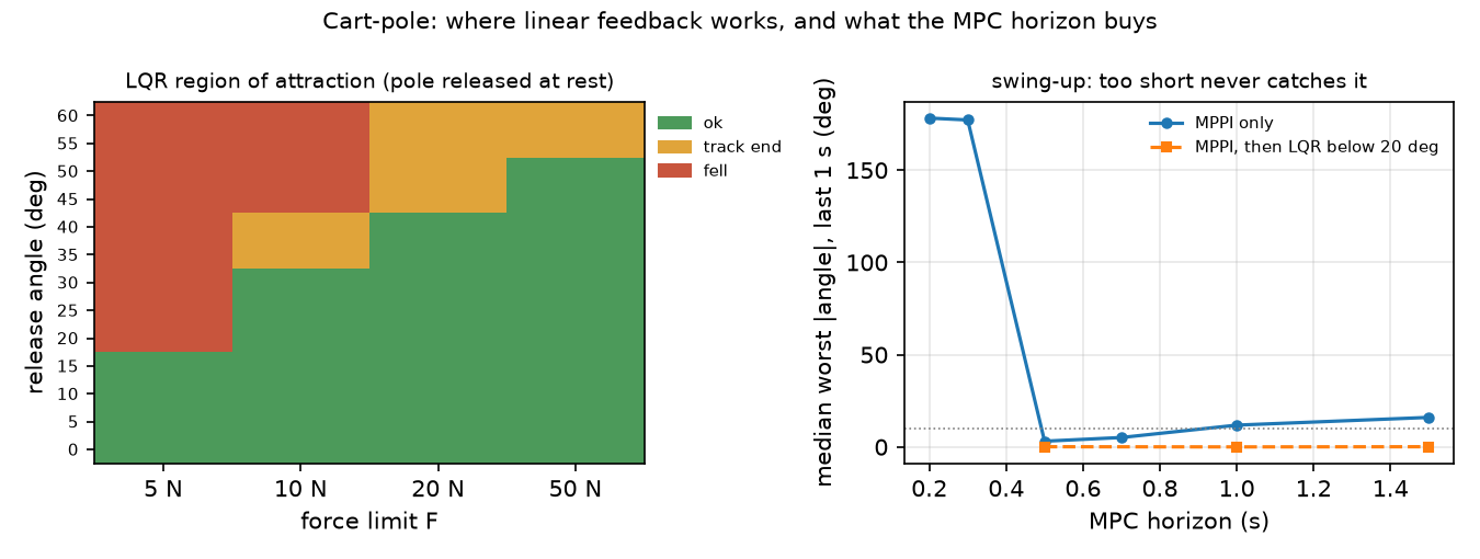
Part B, region of attraction. Release the pole at rest at $\theta_0$ , cart at $x=0$ , apply $u = \text{clip}(-K\delta x, \pm F)$ for 5 s; success is $\lvert\theta\rvert < 2°$ at the end. Prediction: larger force limits help, but only up to a point.

$\theta_0$ (deg)	F = 5 N	F = 10 N	F = 20 N	F = 50 N
0–15	ok	ok	ok	ok
20–30	fell	ok	ok	ok
35–40	fell	track end	ok	ok
45–50	fell	fell	track end	ok
55–60	fell	fell	track end	track end
180 (down)	not up	not up	not up	not up

Two failure modes. With a small force limit the linear law asks for more force than exists, the command saturates and the pole falls. With enough force the pole is caught, but the cart hits the track end: LQR knows a quadratic penalty on $x$ , not the constraint $\lvert x\rvert \le 1.5$ m. From hanging down (a trial that cannot “fall” and runs the full 5 s) LQR never brings the pole up: the linearization at the upright says nothing there.

Part C, MPPI swing-up. From hanging down, $\lvert F\rvert \le 20$ N, 64 samples, $\sigma = 8$ N, $\lambda = 0.5$ , 50 Hz, 6 s, 8 seeds per row; sweep the horizon. “Held” means $\lvert\theta\rvert < 10°$ for the whole last second; “worst” is the median over seeds of the largest $\lvert\theta\rvert$ in it.

horizon (s)	steps	passed upright	held	median first time up (s)	worst $\lvert\theta\rvert$ , last 1 s (deg)	median cost
0.2	10	8/8	0/8	0.80	178.2	30.97
0.3	15	8/8	0/8	0.72	177.2	29.84
0.5	25	8/8	8/8	0.90	3.1	10.79
0.7	35	8/8	8/8	1.27	5.1	9.12
1.0	50	8/8	3/8	1.09	11.8	7.57
1.5	75	8/8	1/8	1.51	16.0	10.08

Too short (0.2–0.3 s): the pole passes upright but is never caught (178.2° in the last second): the controller cannot see far enough to brake in time.
0.5–0.7 s: swing-up and balance in all 8 seeds (3.1°, 5.1°).
Longer (1.0–1.5 s): still swings up every time and 1.0 s gives the lowest median cost (7.57), but balance gets sloppy (11.8°, 16.0°). Consistent with these numbers, not confirmed by a sample-count sweep: 64 samples cover a 50- or 75-step sequence more sparsely, so the averaged first input is noisier.

The engineering answer: use both. Switch from MPPI to the LQR once $\lvert\theta\rvert < 20°$ :

horizon (s)	passed upright	held	median first time up (s)	worst $\lvert\theta\rvert$ , last 1 s (deg)	median cost
0.5	8/8	7/8	1.09	0.1	7.61
1.0	8/8	8/8	1.12	0.0	7.16
1.5	8/8	8/8	1.66	0.1	9.00

MPC does the nonlinear part, LQR holds the equilibrium with a precision sampling cannot match. One 0.5 s run did not hold; likely (not isolated) because Part B measured the region at rest and a hand-off happens at speed.

Left: LQR outcomes by release angle (0 to 60 degrees) and force limit (5 to 50 N); the region that ends upright grows with the force limit, bounded by falls and then by the track end. Right: median worst pole angle in the last second against the MPC horizon: 178.2 and 177.2 degrees at 0.2 and 0.3 s, 3.1 degrees at 0.5 s, 16.0 degrees at 1.5 s; with the LQR hand-off 0.1 degrees or less.

Break it

The break is in the tables: the LQR region ends where the force saturates or the track ends (Part B); MPPI breaks at both ends of the horizon sweep (Part C). When each suffices:

situation	LQR	MPC
small deviations around one equilibrium, inputs well inside limits	sufficient and cheapest (one matrix-vector product)	unnecessary
large deviations, nonlinear motion (swing-up)	fails (180°: not up at any force)	needed
hard constraints (force, track, contacts)	ignored, only penalized through $Q$ , $R$	in the cost or as constraints
compute per step	$O(n\,m)$	$K$ rollouts of $H$ steps (here 64 rollouts of up to 75 control steps)

On the real robot

MPC runs on real legged robots. The MIT Cheetah 3 controller simplifies the dynamics until the problem is convex, predicts up to 0.5 s and solves in under 1 ms at 20–30 Hz (Di Carlo et al., IROS 2018): simplify the model until the solver meets the control period.
SO-101. The Menagerie model drives every joint through position servos (kp="998.22" kv="2.731", force limit ±2.94 N·m, so101.xml), so mjd_transitionFD’s $B$ maps position targets, not torques, to the next state. Design an LQR on that servo-in-the-loop model, simulate it with the force clip, then test it at low gain on the arm. Not yet measured on the real arm.
The region of attraction must be measured. Our table is a simulation with an exact model; delays, friction and estimation noise shrink it on hardware. Sweep the initial condition on the real system, velocity included.

Check yourself

Quick check · 2 questions. Click an answer.

1. Part B: with F = 5 N the LQR fails from 20° as “fell”; with F = 10 N the failures at 35–40° are “track end”. What explains the two modes?

Both come from a bad linearization at the upright.
At 5 N the command saturates and the pole falls; at 10 N the pole is caught, but LQR only penalizes cart position through $Q$ and does not know the track ends.
At 10 N the controller is too aggressive and overshoots; lowering every entry of $Q$ fixes both.

Why: Part B table and text: the constraint $\lvert x\rvert \le 1.5$ m is not in the LQR. Even at 50 N the region ends between 50° and 55°.

2. MPPI alone with a 0.2 s horizon passes upright 8/8 but holds 0/8. What does that show, and what worked best?

The horizon is too short to see far enough ahead to brake; MPPI for the swing-up plus an LQR hand-off below 20° held 8/8 at 1.0 and 1.5 s.
The horizon is too long, so the samples cover it too thinly; 0.1 s would hold.
64 samples are too many; fewer samples would average less noise into the plan.

Why: Part C: worst angle in the last second 178.2° at 0.2 s, held 8/8 at 0.5–0.7 s; with the hand-off the worst angle was 0.0° at 1.0 s and 0.1° at 1.5 s.

Easy. Why does LQR started from hanging down fail regardless of the force limit?
Medium. With F = 10 N the failures at 35–40° are “track end”. Which entry of $Q$ would you raise, and what do you expect to happen to the “fell” boundary?
Hard. Test the explanation for the long-horizon wobble: at a 1.0 s horizon, sweep the sample count (64, 128, 256) and measure “held” and the worst angle.

Answers

The linear model is valid only near $\theta = 0$ . Near $\theta = \pi$ the coupling from cart force to pole acceleration ( $\propto \cos\theta$ ) has the opposite sign, and a fixed linear law cannot pump energy into a swing. Measured: “not up” at all four forces.
The cart-position weight $Q_{11}$ . The cart stays nearer the centre at the price of a more aggressive pole recovery, so some track-end cases may become “fell” at 10 N. Not computed here.
Not computed here; run it.

Takeaways and sources

Linearize, iterate Riccati, done: an LQR from any MuJoCo model in a few lines. It caught the pole up to 15° at 5 N and up to 50° at 50 N, and failed by saturation or at the track end beyond.
MPPI swung the pole up in 8/8 seeds at every horizon but held it only at 0.5–0.7 s with 64 samples.
MPC for the swing-up plus LQR for the balance held 8/8 at 1.0 and 1.5 s, worst angle at most 0.1°.

Next: lesson 25, how to evaluate a policy with enough trials to trust the success rate.

Sources

R. Tedrake, Underactuated Robotics, ch. 8 “Linear Quadratic Regulators” (lqr.html) and ch. 10, section on model-predictive control (trajopt.html).
MuJoCo API reference, mjd_transitionFD; Python bindings, mujoco.rollout.
SciPy, scipy.linalg.solve_discrete_are.
G. Williams et al., “Information Theoretic MPC for Model-Based Reinforcement Learning”, ICRA 2017. PDF.
J. Di Carlo, P. M. Wensing, B. Katz, G. Bledt, S. Kim, “Dynamic Locomotion in the MIT Cheetah 3 Through Convex Model-Predictive Control”, IROS 2018. MIT DSpace.
All tables: experiments/24-lqr-and-mpc/output.txt (MuJoCo 3.17.0, 2026-10-27).