30 · Multimodal actions: diffusion and flow policies

Part	7 · Learning from demonstration
Run type	CPU · Mac or Colab CPU
Prerequisites	28
Learn first	Diffusion Models — DDPM from Scratch · Flow Matching & Rectified Flows · Loss Functions
Time	~75 min
Code	experiments/30-diffusion-and-flow-policies/experiment.py · notebook
Status	✅ done

Act on this lesson

Tick each step when you have done it. Saved in this browser only.

1. 01 · Read The problem and the core idea; answer the questions before you read.
2. 02 · Build it Type the steps yourself, then run uv run python experiments/30-diffusion-and-flow-policies/build.py
3. 03 · Run the experiment Predict first, then run uv run python experiments/30-diffusion-and-flow-policies/experiment.py
4. 04 · Break it Change the one parameter and watch it fail.
5. 05 · Check yourself Quizzes and exercises at the end.

Mark lesson complete

A regression policy returns the average of the demonstrations. When the demonstrations disagree, the average can be the one motion nobody showed.

The problem

Diffusion Policy (Chi et al. 2023) starts from multimodal actions: in one state there can be several correct motions, each a “mode”. In their Push-T task the policy “learns to approach the contact point equally likely from left or right”, while LSTM-GMM and IBC show a bias toward one side and BET “cannot commit to one mode” (Sec. 5.3).

The smallest version of that failure: a point must go from $(0,-1)$ to $(0,+1)$ past a round obstacle of radius 0.30 at the origin. Of 200 demonstrations, 100 pass on the left and 100 on the right, whatever the start. A behavior-cloning MLP (lesson 28) trained with MSE on them collides in 200 of 200 trials in simulation. Why, and what replaces it?

Before you read · 2 questions. Guess first; the lesson tells you why.

1. 100 demonstrations pass left of the obstacle and 100 pass right. Why does the MSE policy collide in 200 of 200 trials?

• MSE learns the conditional mean; the average path passes at $x = +0.030$, inside the obstacle radius of 0.30.
• The network is too small to fit 200 demonstrations.
• MSE always picks the left mode, and the obstacle sits slightly to the left.

Why: Part A: the demonstrations pass at −0.55 and +0.55. More data makes it worse: 8% collisions with 10 demos, 100% with 200 and 500 (part B).

2. A generative policy answers by starting from random noise and pushing it, step by step, until it looks like a demonstration. With half the demonstrations passing left and half right, what decides which side one answer takes?

• The observation alone; every query from the same start gives the same path.
• Nothing; it always returns the average of both sides.
• Where the random start lies; different noise can end on different sides, each about as often as in the data.

Why: Plain words and Part C; at 32 Euler steps the flow policy passed 97 times left and 100 times right of 200 trials, without being told there are two modes.

Core idea

In plain words

Two equally good roads go around a field, left and right, and half of the drivers you learn from take each. Train a navigator to give one answer as close as possible, on average, to what the drivers did, and it answers with the midpoint: straight through the field. That is what regression with an MSE loss does: it returns the average of the demonstrations, fine when they agree, wrong when they split.

The fix is to learn to sample an answer: each query returns one plausible road, about as often as the drivers chose each. A mixture model predicts a fixed number of candidates plus their probabilities and picks one. Generative models (diffusion, flow matching) need no fixed number: they start from random noise and push it, step by step, until it looks like a demonstration; flow matching learns the push as a velocity field, and the random start decides the road. The number of pushes is a knob: many small pushes follow the flow to one road, one big push lands on the average, back in the field.

flowchart TD
    O["observation o<br/>(start point)"] --> M{"how is the path produced?"}
    M -->|"MSE regression"| A["one answer:<br/>the average path"]
    A --> X["through the obstacle"]
    M -->|"flow matching"| Z["random noise a0"]
    Z --> V["N small pushes along the<br/>learned velocity v(a, t, o)"]
    V --> S["one sampled path:<br/>left or right"]

Flow matching as code

# MSE regression, for comparison: one answer per observation -> learns E[a1 | o]
loss_mse = ((net_mse(o) - a1) ** 2).mean()

# flow matching, one training step
a1, o = sample_demos(batch)               # demonstrated path (80 numbers) and its observation
a0 = torch.randn_like(a1)                 # pure noise with the same shape
t = torch.rand(batch, 1)                  # random time in [0, 1]
at = (1 - t) * a0 + t * a1                # a point on the straight line from noise to demo
target = a1 - a0                          # the velocity of that straight line
loss = ((net(at, t, o) - target) ** 2).mean()   # still MSE, but on velocities, not on paths

# sampling: Euler integration from noise (t = 0) to a path (t = 1)
def sample(net, o, n_steps):
    a = torch.randn(80)                   # a different random start can end on the other side
    for i in range(n_steps):
        a = a + net(a, i / n_steps, o) / n_steps   # one small push along the learned velocity
    return a

What	Formula
MSE optimum	$f^*(o) = \mathbb{E}[a \mid o]$; two 50/50 modes give $\tfrac12(a_L + a_R)$
Mixture model	$p(a \mid o) = \sum_k \pi_k(o)\,\mathcal N(a;\mu_k(o), \sigma^2 I)$
Flow-matching loss	$a_t = (1-t)\,a_0 + t\,a_1, \quad \mathcal L = \mathbb{E}\,\bigl\lVert v_{\theta}(a_t, t, o) - (a_1 - a_0)\bigr\rVert^2$
Sampling (Euler)	$a \leftarrow a_0, \quad a \leftarrow a + \tfrac1N\, v_{\theta}\!\left(a, \tfrac iN, o\right), \quad i = 0,\dots,N-1$

$o$ is the observation (here the start point), $a$ the action (here the whole path), $a_L$ and $a_R$ the left and right demonstrated paths, $\pi_k$, $\mu_k$ and $\sigma$ the weight, mean and fixed spread of mixture component $k$ out of $K$, $a_0 \sim \mathcal N(0, I)$ the noise, $a_1$ a demonstration, $t \sim U(0,1)$ the time along the path from noise to data, $v_\theta$ the learned velocity network and $N$ the number of Euler steps (each one network call).

Math details: why MSE averages, and why one Euler step is regression again

MSE learns the conditional mean. For any $f$, $\mathbb{E}\,\lVert a - f(o)\rVert^2 = \mathbb{E}\,\lVert a - \mathbb{E}[a\mid o]\rVert^2 + \mathbb{E}\,\lVert \mathbb{E}[a\mid o] - f(o)\rVert^2$; the first term does not depend on $f$, so the minimizer is $f^*(o) = \mathbb{E}[a \mid o]$ (see AIEFS: Loss Functions). With two equally likely modes this is the middle of the obstacle. An L1 loss gives the per-dimension median instead; with exactly 50/50 modes any point between them is a median, so it is no better (L1 returns in lesson 31).

Mixture model. Train by negative log-likelihood; at run time sample $k$ from $\pi_k(o)$, then output $\mu_k$. It works if you know $K$ and the components do not collapse. Generative action models sample from $p(a \mid o)$ without fixing $K$; $a$ is usually a whole chunk of future actions and $o$ a condition. We implement flow matching with straight paths ($\sigma_{\min} = 0$).

One step is regression. At $t = 0$, $a_t = a_0$ carries no information about $a_1$, so the best velocity is $v^*(a_0, 0, o) = \mathbb{E}[a_1 \mid o] - a_0$. A single Euler step lands on $a_0 + v^* = \mathbb{E}[a_1 \mid o]$, the MSE answer. Later steps see an $a_t$ that already leans to one side, and the learned velocity bends toward that side’s mode. The integration steps are what turn regression into sampling.

Go deeper (AIEFS): Diffusion Models — DDPM from Scratch, Flow Matching & Rectified Flows, Loss Functions. Primary sources: Lipman et al. 2023, Ho et al. 2020, Chi et al. 2023.

Four ways to produce an action

	trained to predict	sampling	cost per action
MSE regression	$\mathbb{E}[a\mid o]$	none	1 network call
Mixture (MDN)	$\pi_k, \mu_k$	pick $k$, take $\mu_k$	1 call
DDPM (Ho et al. 2020)	the noise $\epsilon$ added to $a$, given $(a_t, t, o)$	start from Gaussian noise, denoise $N$ times	$N$ calls
Flow matching (Lipman et al. 2023)	a velocity field $v_{\theta}(a_t, t, o)$	integrate an ODE from noise in $N$ steps	$N$ calls

DDPM (“denoising diffusion”) and flow matching are close relatives: both start from noise and need $N$ network calls per sample; flow matching regresses a velocity, DDPM the noise to remove.

Build it

You will now write the three pieces of a flow policy, the training pair, the velocity field and the Euler sampler, and check each on the Experiment’s 200 demonstrations and 200 trials. Instead of training a network, you derive the field a perfect network would learn on these demonstrations: no PyTorch, about 2 s, and it separates what flow matching does from what a learned network adds.

The functions are in physai/imitation.py; uv run python experiments/30-diffusion-and-flow-policies/build.py runs the four steps (output in build_output.txt).

Step 1 · The least-squares answer is the mean

Fit the paths by least squares, linear in the start $x_0$, which is the best MSE predictor for this data:

F = np.c_[np.ones(len(X)), X[:, 0]]                 # 1 and the start x0 of each demonstration
coef = np.linalg.lstsq(F, Y, rcond=None)[0]         # 80 path numbers, linear in x0

== Step 1. 200 demonstrations, half left, half right: the least-squares answer ==
demos pass the obstacle (y = 0) at x = -0.551 / +0.552
least-squares path from x0 = 0 passes at x = +0.000; max |intercept - mean of the 200 demos| = 7.5e-15
200 trials: collided 200/200, left 0, right 0

The intercept is the mean of the 200 demonstrations (difference 7.5e-15); the path passes the obstacle at $x = +0.000$, dead centre: 200/200 collisions. The Experiment’s MSE network approximates this mean (200/200, path at $+0.030$).

Step 2 · The training pair and what it regresses

def flow_matching_pair(a0, a1, t):
    """Training input and target of flow matching with straight paths: a_t on the line noise -> data, and its velocity."""
    t = np.reshape(t, (-1,) + (1,) * (np.ndim(a1) - 1))
    return (1 - t) * a0 + t * a1, a1 - a0

A network sees only $a_t$, not which $a_0$ and $a_1$ produced it, so the best it can learn is the average target over all pairs passing through $a_t$. For a finite dataset that average has a closed form: given demonstration $j$, $a_t$ is Gaussian around $t\,a^{(j)}$ with standard deviation $1 - t$, so the posterior over $j$ is a softmax, and each demonstration pulls with velocity $(a^{(j)} - a)/(1 - t)$:

def empirical_velocity(a, t, data):
    """The velocity field that minimizes the flow-matching loss on a finite dataset: E[a1 - a0 | a_t = a].

    Given a1 = data[j], a_t is Gaussian around t * data[j] with std (1 - t), so the posterior over j is a softmax.
    a: (n, D) points at time t (0 <= t < 1); data: (m, D) demonstrations.
    """
    a = np.atleast_2d(a)
    d2 = ((a[:, None, :] - t * data[None, :, :]) ** 2).sum(-1)      # (n, m) squared distances
    logw = -d2 / (2 * (1 - t) ** 2)
    w = np.exp(logw - logw.max(1, keepdims=True))
    w /= w.sum(1, keepdims=True)
    return (w @ data - a) / (1 - t)                                 # sum_j w_j (data_j - a) / (1 - t)

The check draws 4 million pairs from two 1-D modes at $\pm 1.1$ (the obstacle offsets $\pm 0.55$ times the Experiment’s scaling of 2) and averages the target near five points at $t = 0.5$:

== Step 2. The flow-matching pair and the field it regresses ==
t = 0.0: a_t = [0.3 0.3], target a1 - a0 = [ 0.8 -1.4]
t = 0.5: a_t = [ 0.7 -0.4], target a1 - a0 = [ 0.8 -1.4]
t = 1.0: a_t = [ 1.1 -1.1], target a1 - a0 = [ 0.8 -1.4]
t = 0.5     a    mean target near a (Monte Carlo)   empirical_velocity
         -0.8                          -0.467               -0.474
         -0.2                          -0.501               -0.510
         +0.0                          -0.001               +0.000
         +0.2                          +0.524               +0.510
         +0.8                          +0.478               +0.474

Monte Carlo agrees within about 0.015, its sampling noise. At $a = 0$ the two modes pull equally; a little to either side the field already points to that side’s mode.

Step 3 · Euler sampling

def euler_sample(velocity, a0, n_steps):
    """Integrate da/dt = velocity(a, t) from t = 0 (noise a0) to t = 1 in n_steps equal Euler steps."""
    a = np.array(a0, dtype=float)
    for i in range(n_steps):
        a = a + velocity(a, i / n_steps) / n_steps
    return a

Integrate the exact field of the 200 demonstrations from noise, with the Experiment’s trials, and compare with the Experiment’s learned network:

== Step 3. Euler sampling along the exact field of the 200 demonstrations ==
steps  collided  left  right  mean |x| at y=0   (Experiment's network: collided, mean |x|)
    1   200/200     0      0            0.026   (200/200, 0.161)
    2    34/200    84     82            0.403   (95/200, 0.372)
    4     0/200    98    102            0.487   (17/200, 0.494)
    8     0/200    97    103            0.515   (7/200, 0.533)
   16     0/200    97    103            0.528   (5/200, 0.546)
   32     0/200    97    103            0.536   (3/200, 0.554)
1 step: max |sample - mean of the demos| = 3.0e-14

One step lands exactly on the mean of the demonstrations (3.0e-14) and collides 200/200: “one step is regression” (Math details), measured. With 2 steps 34 samples still end between the modes (the network: 95); from 4 steps on the exact field never collides, while the network still does (17, 7, 5, 3). The gap is the network’s error.

Step 4 · What a perfect fit does

== Step 4. Many steps: the exact field returns the training demonstrations ==
   8 steps: RMS distance of a sample to its nearest demonstration, median 0.0018, max 0.0158
  32 steps: RMS distance of a sample to its nearest demonstration, median 0.0009, max 0.0029
 128 steps: RMS distance of a sample to its nearest demonstration, median 0.0000, max 0.0010
demonstrations differ from each other by (median RMS, nearest pair) 0.0024

After 128 steps every sample sits on one of the 200 demonstrations (median RMS distance 0.0000; neighbouring demonstrations differ by 0.0024): the exact minimizer of the training loss memorizes the data. A network smooths this field and produces new paths between nearby demonstrations, which is why it generalizes and why it leaves a few samples between the modes.

What you keep

physai.imitation now also has flow_matching_pair, empirical_velocity and euler_sample; euler_sample takes any velocity function, so the same sampler runs a trained network. Lesson 31 keeps the chunked action and drops the sampler; lesson 41 meets flow-matching action heads again in vision-language-action models. tests/test_30_diffusion_and_flow_policies.py checks the one-step mean, that a single demonstration is reached exactly in any number of steps, and that many steps land on a mode; run uv run pytest tests/test_30_diffusion_and_flow_policies.py.

Use it

For a real arm, LeRobot’s Diffusion Policy is ready-made: lerobot-train --policy.type=diffusion. It is DDPM, not flow matching, but the knobs are the ones you built (configuration_diffusion.py):

Knob	This lesson	LeRobot DiffusionConfig default
what the network predicts	velocity $a_1 - a_0$	prediction_type = "epsilon" (the added noise)
steps per sample (network calls)	n_steps, 1 to 32	num_inference_steps, defaults to num_train_timesteps = 100
sampler	Euler, $t$: 0 → 1	noise_scheduler_type = "DDPM"
action chunk	the whole path, 40 waypoints	horizon = 64 predicted, n_action_steps = 32 executed
observation	the start point	n_obs_steps = 2 (current and previous step)
action normalization	divide by SCALE = 2	MIN_MAX for state and action, then clip_sample_range = 1.0

Three traps:

• Noise and data must have comparable scale. The sampler starts from $\mathcal N(0, I)$; the Experiment multiplies paths by 2 so that offsets of about 0.5 become about 1. Unnormalized actions in radians or millimetres make the first steps meaningless.
• Time runs in opposite directions. Here (and in Lipman et al.) $t = 0$ is noise and $t = 1$ is data; DDPM counts its timesteps down from noise at $T$ to data at 0. Mixing the conventions integrates the wrong way.
• Steps cost latency. Every step is one network call: 100 by default in LeRobot’s diffusion config, against the 0.04–0.77 ms per query of the Experiment’s small MLP at 1–32 steps. Check the budget against your control rate before you choose a step count.

Check after building · 2 questions.

1. In Build it, Step 3, the exact velocity field of the 200 demonstrations collides 0/200 from 4 Euler steps on, while the Experiment’s network still collides 17, 7, 5 and 3 times at 4 to 32 steps. What does that tell you?

• Flow matching itself leaves samples between the modes, whatever the network.
• The remaining collisions come from the network’s approximation of the field, not from flow matching.
• Euler integration is wrong and should be replaced by an exact solver.

Why: One step of the exact field lands on the mean of the demonstrations (difference 3.0e-14) and collides 200/200, like MSE; with more steps it reaches the demonstrations themselves (Step 4).

2. You move to LeRobot’s Diffusion Policy and keep its defaults. How many network calls does one action chunk cost at inference?

• One, because DDPM predicts the action directly.
• Two, one per observation step.
• 100, because num_inference_steps defaults to num_train_timesteps = 100.

Why: Every denoising step is one network call (Use it, the table). Check that budget against the control rate; the Experiment’s small MLP took 0.04–0.77 ms per query at 1–32 steps.

Experiment

Full script: experiments/30-diffusion-and-flow-policies/experiment.py. NumPy 2.5.4, PyTorch 2.14.1 (CPU, 2 threads), Apple Silicon Mac (Apple M5), fixed seeds, deterministic. Parts A–B port the experiment of the earlier notebook and reproduce the numbers recorded for it, except the three-seed MSE check, which now gives somewhat different collision counts.

The observation is the start point $(x_0, y_0)$ with $x_0 \in [-0.05, 0.05]$; the action is the whole path, 40 waypoints relative to the start (80 numbers). A trial passes or hits the obstacle; “left/right” counts the collision-free trials by the side they passed. 200 trials per row, 95% Wilson intervals (lesson 25).

Prediction: the MSE path goes through the middle; the mixture and the flow policy split roughly 50/50.

a0 = torch.randn(a1.shape)                          # noise
t = torch.rand(batch)
at = (1 - t[:, None]) * a0 + t[:, None] * a1        # point on the straight path
loss = ((net(at, t, o) - (a1 - a0)) ** 2).mean()    # regress the velocity, conditioned on o

a = torch.randn(n, 80)                              # sampling: Euler from t = 0 to 1
for i in range(n_steps):
    a = a + net(a, torch.full((n,), i / n_steps), o) / n_steps

Part A. NumPy MLP 64-64 tanh, 1,500 full-batch Adam epochs; mixture with $K = 2$, fixed $\sigma = 0.2$.

model	collided	95% CI	left	right
MSE, demos half left / half right	200/200	98.1–100%	0	0
MSE, all demos on the left	0/200	0–1.9%	200	0
Mixture (MDN, $K=2$)	0/200	0–1.9%	96	104

At $y = 0$ the demonstrations pass at $x = \pm 0.55$, the MSE path at $x = +0.030$, inside the radius of 0.30. With three other seeds the MSE model collided 193, 184 and 200 times out of 200, the mixture 0 times in each.

Part B: more data does not help. Same MSE model, demonstrations half/half:

demos	10	20	50	100	200	500
MSE collisions	8.0%	46.0%	85.0%	91.5%	100%	100%

A likely reason (not instrumented): with 10 demonstrations the network ties tiny differences in $x_0$ to the nearest demonstration’s side; with more data it approaches the conditional mean.

Part C: flow-matching policy on the same 200 demonstrations: MLP 3×256 SiLU, input = noisy chunk + sinusoidal time embedding + observation, 4,000 Adam steps, batch 256. Sweep the number of Euler steps.

Euler steps	collided	95% CI	left	right	single-query time (ms)	mean $\lvert x\rvert$ at $y=0$
1	200/200	98.1–100%	0	0	0.04	0.161
2	95/200	40.7–54.4%	53	52	0.06	0.372
4	17/200	5.4–13.2%	87	96	0.10	0.494
8	7/200	1.7–7.0%	95	98	0.19	0.533
16	5/200	1.1–5.7%	96	99	0.39	0.546
32	3/200	0.5–4.3%	97	100	0.77	0.554

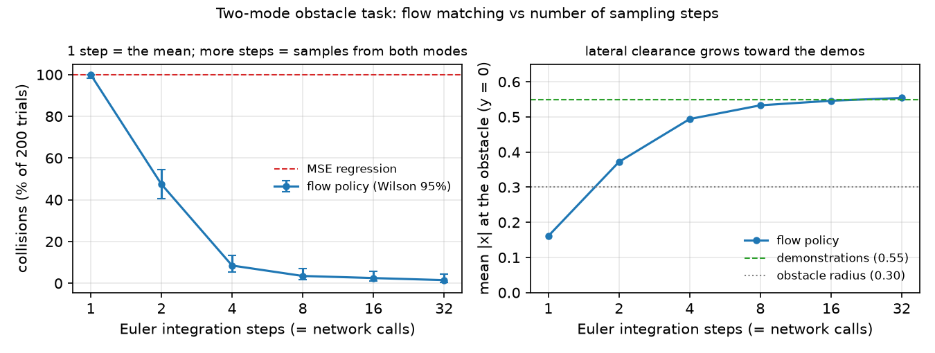
Times are the fastest of 30 single-trajectory queries on a heavily loaded machine (approximate); the step count is the machine-independent cost. The flow policy splits left/right like the mixture model without being told there are two modes, and the lateral offset approaches the demonstrations’ 0.55 as steps increase.

Break it

Cut the integration steps. With 1 step the flow policy collides 200/200, like MSE: mean distance from the centre line 0.161, inside the obstacle. That is the $t = 0$ argument, measured; the paths are not exactly the mean (the exact field of Build it, Step 3 gives 0.026, the spread of the starts) because the learned field still depends a little on $a_0$. With 2 steps 95/200 still end between the modes, and even at 32 steps 3/200 touch the obstacle: the exact field reaches 0/200 from 4 steps on, so what remains is the learned field’s error.

The second break is the data, for the MSE model (200 demos, Part B sweep):

fraction of left demos	50%	60%	70%	80%	90%	100%
MSE collisions	100%	91.5%	63.0%	36.5%	0%	0%

MSE is safe only for nearly unimodal data: the mean lateral offset $0.55\,\lvert 2p_{\text{left}} - 1\rvert$ must clear the radius 0.30 plus a margin.

On the real robot

• Diffusion Policy uses a DDPM to model $p(A \mid O)$, the action sequence conditioned on observations, not their joint distribution; the CNN variant conditions through FiLM (a learned per-channel scale and shift computed from the observation). With DDIM (a faster DDPM sampler), 100 training iterations and 10 inference iterations give about 0.1 s inference on an Nvidia 3080 in their real-world setup; an action horizon of 8 steps worked best for most tasks; reported average improvement 46.9% over prior methods across 15 tasks from 4 benchmarks (Chi et al. 2023).
• π0 uses conditional flow matching for actions, a 300M-parameter “action expert” on a 3B vision-language model (3.3B total), chunks of $H = 50$ actions, 10 integration steps; on an RTX 4090 the 10 action passes take 27 ms of a 73 ms on-board inference (Black et al. 2024). Same trade-off as Part C, at real scale.
• SO-101 procedure (LeRobot’s defaults are in Use it). Record teleop demos of a task with two valid strategies (grasp a cube from either side), train an MSE behavior-cloning baseline and a diffusion policy on the same episodes, and count grasps that end between the two strategies over at least 50 trials each. Not yet measured on the real arm.

Check yourself

Quick check · 2 questions. Click an answer.

1. The flow policy collides 200/200 with 1 Euler step and 3/200 with 32. Why does one step behave like regression?

• One step removes the noise, so every sample is the same.
• At $t = 0$ the input $a_0$ says nothing about the demonstration, so the best velocity is $\mathbb{E}[a_1 \mid o] - a_0$ and one step lands on $\mathbb{E}[a_1 \mid o]$.
• The network was trained only for 32-step sampling.

Why: Math details, “One step is regression”; part C: 200/200 at 1 step, 95/200 at 2, 7/200 at 8 and 3/200 at 32, with cost growing linearly in the steps.

2. Now 80% of the demonstrations pass left. What happens to the MSE policy?

• It never collides, because the average now lies on the left.
• It still collides every time, as at 50/50.
• It collides in 36.5% of trials: the mean passes at about −0.33, just outside the radius 0.30, and jitter pushes many trials inside.

Why: Break it table (50%: 100%, 80%: 36.5%, 90%: 0%); the mean offset $0.55\,\lvert 2p_{\text{left}} - 1\rvert$ must clear the radius plus a margin.

1. Easy. Why does a 1-step flow policy behave like MSE regression?
2. Medium. With 80% left demonstrations, where does the MSE path pass at $y = 0$, and why do some trials still collide?
3. Hard. Write a closed-loop step policy (current position → next step) trained with MSE on the same demonstrations and measure its collision rate. Is the average flow at the centre line stable?

Answers

1. At $t=0$ the input $a_0$ is independent of the target, so the optimal velocity is $\mathbb{E}[a_1\mid o] - a_0$ and one Euler step returns $\mathbb{E}[a_1\mid o]$. Measured: 200/200 collisions, same as MSE.
2. Around $0.8\cdot(-0.55) + 0.2\cdot 0.55 = -0.33$, just outside the radius 0.30; jitter in the learned path and in $x_0$ pushes many trials inside. Measured: 73/200 (36.5%).
3. Not computed here; run it.

Takeaways and sources

• MSE regression returns the conditional mean; with two 50/50 modes it collided 200/200 in simulation, and more data (10 → 500 demos) raised the collision rate from 8% to 100%.
• A mixture model (0/200, 96 left / 104 right) and a flow-matching policy (3/200 at 32 steps, 97 / 100) represent both modes; the flow policy did not need to know the number of modes.
• Sampling steps are the knob: 1 step reproduced the mean (200/200), 8 steps reached 7/200, and cost grows linearly with steps.

Next: lesson 31, predicting chunks of future actions and executing them.

Sources

• C. Chi et al., “Diffusion Policy: Visuomotor Policy Learning via Action Diffusion”, 2023. arXiv 2303.04137.
• K. Black et al., “π0: A Vision-Language-Action Flow Model for General Robot Control”, 2024. arXiv 2410.24164.
• Y. Lipman, R. T. Q. Chen, H. Ben-Hamu, M. Nickel, M. Le, “Flow Matching for Generative Modeling”, 2023. arXiv 2210.02747.
• J. Ho, A. Jain, P. Abbeel, “Denoising Diffusion Probabilistic Models”, 2020. arXiv 2006.11239.
• LeRobot, configuration_diffusion.py.
• All tables: experiments/30-diffusion-and-flow-policies/output.txt (2026-10-27).