09 · Jacobians and differential kinematics


Part	3 · Kinematics
Run type	CPU · Mac or Colab CPU
Prerequisites	08
Learn first	Calculus for Machine Learning · Linear Systems
Time	~45 min
Code	`experiments/09-jacobians/experiment.py`
Status	✅ done

Act on this lesson

Tick each step when you have done it. Saved in this browser only.

01 · Read The problem and the core idea; answer the questions before you read.
02 · Build it Type the steps yourself, then run uv run python experiments/09-jacobians/build.py
03 · Run the experiment Predict first, then run uv run python experiments/09-jacobians/experiment.py
04 · Break it Change the one parameter and watch it fail.
05 · Check yourself Quizzes and exercises at the end.

One matrix maps joint speeds to tool speed, and its transpose maps tool forces back to joint torques.

The problem

How much torque does the SO-101’s shoulder servo need to hold a 2 N push at the gripper? How fast does the gripper move when the joints turn at a combined 1 rad/s? Both questions have the same answer: a 6×5 matrix that changes with every pose. The Menagerie model limits each servo to 2.94 N m (forcerange="-2.94 2.94" in so101.xml); whether a payload is safe depends on that matrix, not on the payload alone.

You also need that matrix to be exactly right: lesson 10 iterates with it hundreds of times. A common shortcut is to compute it by finite differences. This lesson measures when that shortcut is accurate and when it is not.

Before you read · 2 questions. Guess first; the lesson tells you why.

1. The shoulder turns at the same speed with the arm folded and with it stretched out. When does the gripper move faster?

Folded, because the motor carries less load.
Stretched, because the gripper is farther from the shoulder axis.
The same in both, because the joint speed is the same.

Why: A hinge’s column is $\hat a \times (p - o)$ ; its length grows with the distance from the axis to the tool, like a longer wrench (In plain words).

2. You push straight down on the gripper. Which joint feels no torque from that push?

shoulder_pan, whose axis is vertical.
shoulder_lift, the joint closest to the base.
None; every joint feels part of it.

Why: A vertical force has no moment about a vertical axis. In the Experiment, Step 3, $J^\top F$ for $F = (0, 0, -2)$ N starts with 0.0000.

Core idea

In plain words

Turn one motor a little and watch the gripper: it moves a little in some direction, at some speed. Do that for each motor and write the answers down, one column per motor. That table is the Jacobian: “which way and how fast the hand moves when each motor turns a little”. Turn several motors at once and the hand’s velocity is simply the sum of those columns, each scaled by its motor’s speed. The table changes with the pose, because the lever arms change: the shoulder moves the hand much faster when the arm is stretched out than when it is folded.

The same table, read backwards (its transpose), answers the force question. Push on the gripper and each motor feels a torque equal to the push times its lever arm, which is exactly what its column encodes. A long lever multiplies the torque, like a long wrench.

If you cannot write the table down analytically, you can measure it: nudge one joint by a small step, see how far the tool moved, divide. That is a finite difference, the same trick as a numerical gradient check in ML. Too large a step and the curvature of the motion spoils the estimate; too small and floating-point round-off does.

flowchart TD
    Q["current pose q<br/>(joint angles)"] -.-> J["Jacobian J(q)<br/>6 rows × 5 columns,<br/>one column per joint"]
    QD["joint speeds q̇"] --> M1["multiply by J"]
    J -.-> M1
    M1 --> V["tool velocity:<br/>linear v, angular ω"]
    F["force and moment<br/>at the tool (F, M)"] --> M2["multiply by Jᵀ"]
    J -.-> M2
    M2 --> T["joint torques τ"]

Jacobians as code

import numpy as np

def hinge_column(axis, o, p):    # axis: joint axis (unit, world), o: point on the axis, p: tool point
    jp = np.cross(axis, p - o)   # tool linear velocity per 1 rad/s of this joint (m/s)
    jr = axis                    # tool angular velocity per 1 rad/s of this joint (rad/s)
    return np.r_[jp, jr]

J = np.column_stack([hinge_column(a, o, p) for a, o in zip(axes, origins)])   # 6 x n
twist = J @ qdot                 # [v; w]: tool velocity for joint speeds qdot
tau = J.T @ np.r_[F, M]          # joint torques for the tool to push with force F and moment M

def fd_column(tool_pos, q, i, eps=1e-5):   # central difference for column i (position rows)
    dq = np.zeros_like(q)
    dq[i] = eps
    return (tool_pos(q + dq) - tool_pos(q - dq)) / (2 * eps)

Quantity	Formula
Velocity map	$\begin{bmatrix} v \\ \omega \end{bmatrix} = J(q)\,\dot q = \begin{bmatrix} J_p(q) \\ J_r(q) \end{bmatrix}\dot q ,\qquad J \in \mathbb R^{6\times n}$
Column $i$ of a hinge	$J_{p,i} = \hat a_i \times (p - o_i)$ , $\ J_{r,i} = \hat a_i$
Static force map	$\tau = J^\top \begin{bmatrix} F \\ M \end{bmatrix}$
Forward difference	$\frac{x(q + \varepsilon e_i) - x(q)}{\varepsilon}$ , error $O(\varepsilon)$
Central difference	$\frac{x(q+\varepsilon e_i) - x(q-\varepsilon e_i)}{2\varepsilon}$ , error $O(\varepsilon^2)$

$q$ and $\dot q$ are the joint angles and speeds; $v$ and $\omega$ are the tool’s linear and angular velocity in world coordinates; $J_p$ and $J_r$ are the three position and three rotation rows of $J$ ; $\hat a_i$ is hinge $i$ ‘s unit axis in world coordinates and $o_i$ any point on it; $p$ is the tool point; $F$ and $M$ are the force and moment the tool exerts on the environment; $\tau$ is the vector of joint torques; $x(q)$ is the tool position, $e_i$ the unit vector for joint $i$ and $\varepsilon$ the step.

This is the geometric Jacobian (Lynch & Park, Modern Robotics, Ch. 5). MuJoCo returns it with mj_jac (any world point attached to a body), mj_jacBody and mj_jacSite (API reference). An external wrench (force plus moment) $(F, M)$ pushing on the tool is held by $-J^\top[F;M]$ .

Math details: the column formula, virtual work and the best finite-difference step

Column of a hinge. Turning hinge $i$ at 1 rad/s rotates everything beyond it about the axis $\hat a_i$ through $o_i$ . A point $p$ on a rigid body rotating with angular velocity $\omega$ about a line through $o$ moves with $\omega \times (p - o)$ , which gives $J_{p,i} = \hat a_i \times (p - o_i)$ and $J_{r,i} = \hat a_i$ .

Static force map by virtual work. In equilibrium the power the joints put in equals the power the tool delivers: $\tau^\top \dot q = [F; M]^\top [v; \omega] = [F; M]^\top J\dot q$ for every $\dot q$ , hence $\tau = J^\top [F; M]$ . Friction, backlash and gravity are extra terms (gravity enters in Break it).

Finite-difference error. A Taylor expansion gives a truncation error of order $\varepsilon$ for the forward difference and $\varepsilon^2$ for the central one. Floating-point round-off adds an error of about $\epsilon_{\text{mach}}\lvert x\rvert/\varepsilon$ , where $\epsilon_{\text{mach}}$ is the machine epsilon (the relative precision of a double). Minimizing the sum gives a best step of roughly $\sqrt{\epsilon_{\text{mach}}}$ for forward and $\sqrt[3]{\epsilon_{\text{mach}}}$ for central differences.

Rotation columns are special. Moving one hinge by $\varepsilon$ rotates the tool by exactly $\varepsilon$ about that hinge’s axis, so the orientation difference quotient has no truncation error, only round-off (Experiment, Step 2).

Go deeper: AIEFS Calculus for Machine Learning, Linear Systems; Lynch & Park, Modern Robotics, Ch. 5 “Velocity Kinematics and Statics”.

Build it

You will now write the SO-101’s Jacobian yourself in about 30 lines of NumPy on top of lesson 08, and check every step against MuJoCo. From lesson 08 you have chain_from_mujoco and fk, which returns every hinge’s world axis $\hat a_i$ , a point $o_i$ on it, and the tool point $p$ : exactly the three things the column formula needs. Nothing new comes from MuJoCo.

Type the steps into a file of your own (for example scratch/my_jacobian.py) and run it after each step. The finished functions are in physai/kinematics.py; uv run python experiments/09-jacobians/build.py runs all four steps with the checks (output in build_output.txt).

Step 1 · One hinge column

The formula from Core idea, for one hinge: the linear part is the axis crossed with the lever from the axis to the tool, the angular part is the axis itself.

def hinge_column(axis, o, p):
    """Tool twist per 1 rad/s of one hinge: linear part a x (p - o), angular part a."""
    return np.r_[np.cross(axis, p - o), axis]

chain = chain_from_mujoco(m, "gripperframe")              # lesson 08
axes, anchors, p = fk(chain, Q0)
col = hinge_column(axes[1], anchors[1], p)                # shoulder_lift

== Step 1. One hinge column at q = (0, -0.6, 0.9, 0.4, 0.3) ==
shoulder_lift column, ours:    -0.0198   0.0000  -0.2193   0.0000   1.0000   0.0000
shoulder_lift column, MuJoCo:  -0.0198   0.0000  -0.2193   0.0000   1.0000   0.0000
lever |a x (p - o)| = 0.2202 m, max difference 8.3e-17

The lift column is $(-0.0198, 0, -0.2193)$ m/s per rad/s: turning the lift moves the tool mostly straight down, at the speed of a 0.2202 m lever.

Step 2 · Columns into a Jacobian

One column per hinge, stacked, using the axes and anchors that fk already returns:

def jacobian(chain, q):
    """Geometric Jacobian (6 x n) of the tool point: rows 0-2 linear, rows 3-5 angular, world frame."""
    axes, anchors, p = fk(chain, q)
    return np.column_stack([hinge_column(a, o, p) for a, o in zip(axes, anchors)])

== Step 2. Jacobian from hinge columns vs mj_jacSite (50 poses) ==
max entry error: linear rows 3.9e-16, angular rows 1.0e-15

Step 3 · Use the matrix

With $J$ in hand, the two questions from The problem are one line each:

J = jacobian(chain, Q0)
speed = np.linalg.norm(J[:3] @ (np.ones(5) / np.sqrt(5)))   # tool speed, every joint at 1/sqrt(5) rad/s
tau = J[:3].T @ np.array([0, 0, -2.0])                       # torques for a 2 N push down

== Step 3. Use it at q = (0, -0.6, 0.9, 0.4, 0.3) ==
tool speed for every joint at 1/sqrt(5) rad/s: 0.312 m/s
F =     [0, 0, -2.0] N  ->  J^T F =  0.0000  0.4385  0.5194  0.2586  0.0042 N m
F =      [2.0, 0, 0] N  ->  J^T F =  0.0052 -0.0397 -0.2571 -0.1873 -0.0036 N m
F =      [0, 1.5, 0] N  ->  J^T F = -0.3745  0.0000  0.0000  0.0000  0.0175 N m

The lift torque for the downward push is 2 N times the vertical entry of the lift column from Step 1. Compare with the Experiment’s Step 3 table: the servo held 0.4383 N m at the lift, here you get 0.4385 N m. The 0.0002 is not a bug. The servos give a little under the load, the arm settles at a slightly different pose, and $J$ depends on the pose; at the settled pose the two agree to 4.2e-14. The pan entry is zero for the reason the first exercise asks about.

Step 4 · Check yourself with finite differences

The test you can run on any Jacobian, including one of a learned model: nudge each joint and difference your own forward kinematics.

def fd_jacobian(tool_pos, q, eps=1e-5):
    """Position rows of the Jacobian by central differences of any function q -> tool position."""
    cols = []
    for i in range(len(q)):
        dq = np.zeros(len(q))
        dq[i] = eps
        cols.append((tool_pos(q + dq) - tool_pos(q - dq)) / (2 * eps))
    return np.column_stack(cols)

== Step 4. Central differences of our FK vs our analytic Jacobian (eps = 1e-5) ==
median max entry error: 4.7e-12

That is the error the Experiment’s ε sweep finds for central differences at ε = 1e-5 against mj_jacSite (5.6e-12), now against your own matrix.

What you keep

physai.kinematics now also has hinge_column, jacobian and fd_jacobian. Lesson 10 builds inverse kinematics on them, lesson 14 a task-space controller. tests/test_09_jacobians.py pins them to MuJoCo; run uv run pytest tests/test_09_jacobians.py after you change anything.

Use it

In practice you ask the library for the same matrix. In MuJoCo that is three calls, and the second one is easy to forget:

mujoco.mj_kinematics(m, d)
mujoco.mj_comPos(m, d)                     # mj_jac* reads data that only mj_comPos fills
jacp, jacr = np.zeros((3, m.nv)), np.zeros((3, m.nv))
mujoco.mj_jacSite(m, d, jacp, jacr, site_id)
J = np.r_[jacp, jacr]                      # equals jacobian(chain, q) to 1e-15 (Build it, Step 2)

Other tools return the same information with different conventions. Check which one you have before you mix numbers:

Tool	Call	Row order	Velocity of which point, in which axes
physai	`jacobian(chain, q)`	linear, then angular	the tool point, world axes
MuJoCo	`mj_jacSite(m, d, jacp, jacr, site)`	two 3 × nv arrays	the site, world axes
Pinocchio	`computeFrameJacobian(model, data, q, frame_id, LOCAL_WORLD_ALIGNED)`	linear, then angular	the frame origin, world axes (as above); `LOCAL` uses the frame’s own axes
Modern Robotics	space Jacobian $J_s$ , body Jacobian $J_b$	angular, then linear	$J_s$ : the body point at the space-frame origin; $J_b$ : the body frame’s origin, body axes

Three traps that cost hours:

Columns are degrees of freedom. MuJoCo’s Jacobians have m.nv columns (velocities), not m.nq (positions). They differ as soon as a model has a free or ball joint (a quaternion has 4 numbers but 3 rotational velocities); see lesson 36.
Quaternion order. MuJoCo stores $(w, x, y, z)$ ; SciPy’s Rotation.from_quat expects $(x, y, z, w)$ unless you pass scalar_first=True.
Stale data. mj_jacSite reads positions computed by the last mj_kinematics/mj_forward; change qpos and forget to recompute, and you get the Jacobian of the previous pose without any error.

Check after building · 2 questions.

1. Build it, Step 1: the shoulder_lift column at q = (0, −0.6, 0.9, 0.4, 0.3) has a linear part of length 0.2202 m. What is that number?

The tool speed (m/s) per 1 rad/s of the lift: the lever from the lift axis to the tool.
The length of the upper arm link in the MJCF file.
The rounding error of the hand-written column.

Why: $|\hat a \times (p - o)|$ is the distance from the axis to the tool point; the column matches MuJoCo’s to 8.3e-17, and 2 N times its vertical entry 0.2193 gives the 0.4385 N m of Step 3.

2. Build it, Step 3 gives $J^\top F$ = 0.4385 N m at the lift for a 2 N downward push; the Experiment’s servo held 0.4383 N m. Why the difference?

A bug in the hand-written Jacobian.
Float rounding in the transpose.
The servos give a little under the load, so the arm settles at a slightly different pose, and $J$ depends on the pose.

Why: Step 3 evaluates $J$ at the commanded pose; the Experiment compares at the settled pose, where $J^\top F$ and the servo torque agree to 4.2e-14. The hand-written $J$ matches mj_jacSite to 1.0e-15 at any given pose (Step 2).

Experiment

Script: experiments/09-jacobians/experiment.py. MuJoCo 3.17.0, NumPy 2.5.4, Apple Silicon Mac (Apple M5), deterministic, a few seconds.

mujoco.mj_kinematics(m, d)
mujoco.mj_comPos(m, d)                     # fills the data mj_jac* reads
jp, jr = np.zeros((3, m.nv)), np.zeros((3, m.nv))
mujoco.mj_jacSite(m, d, jp, jr, site_id)   # 3 x nv each, world frame

Predict first. Is a smaller finite-difference step always better? Which step would you pick?

Step 1 · velocity map. 50 random poses, random unit joint velocities. Predicted $J\dot q$ vs the actual site motion over $10^{-6}$ s: max relative error 7.9e-07 (linear) and 3.8e-07 (angular). With every joint at $1/\sqrt5$ rad/s ( $\lvert\dot q\rvert = 1$ ), the median site speed is 0.306 m/s.

Step 2 · sweep the step ε. Median over 50 poses of the largest entry error against mj_jacSite. Orientation differences use mju_subQuat, rotated into the world frame.

ε (rad)	forward $J_p$	forward $J_r$	central $J_p$	central $J_r$
1e-1	1.2e-02	4.8e-15	4.2e-04	2.6e-15
1e-3	1.2e-04	4.5e-13	4.2e-08	2.5e-13
1e-5	1.2e-06	4.7e-11	5.6e-12	2.3e-11
1e-7	1.2e-08	4.5e-09	4.7e-10	2.3e-09
1e-8	9.8e-09	4.4e-08	4.9e-09	2.3e-08
1e-10	9.5e-07	4.4e-06	4.3e-07	2.2e-06
1e-12	8.9e-05	4.6e-04	4.7e-05	2.4e-04
1e-14	8.3e-03	4.5e-02	4.5e-03	2.6e-02

The translational error is V-shaped. To the right of the minimum, truncation (error falls 10× per decade for forward, 100× for central); to the left, round-off (error rises 10× per decade). The best forward step is 1e-8 (error 9.8e-09), the best central step 1e-5 (error 5.6e-12). For comparison, $\sqrt{\epsilon_{\text{mach}}} =$ 1.5e-08 and $\sqrt[3]{\epsilon_{\text{mach}}} =$ 6.1e-06.

Finite-difference Jacobian error versus step size on log axes. For the translational columns both schemes trace a V: the forward difference is best near 1e-8 rad, the central difference near 1e-5 rad, and both get worse for smaller steps. For the rotational columns the error only grows as the step shrinks.

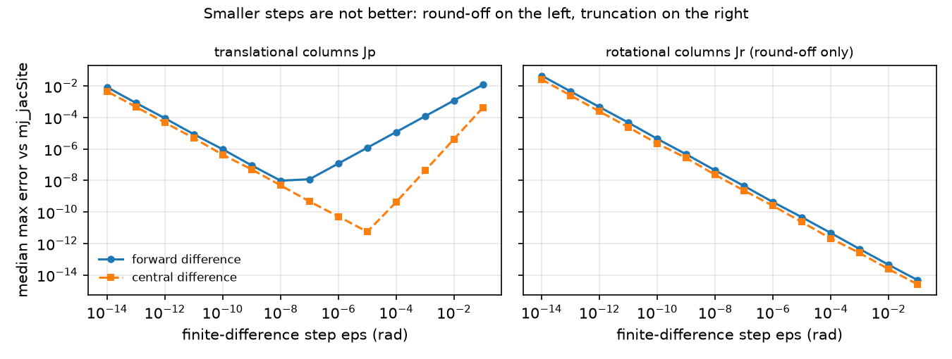
The rotational columns have no truncation error at all: moving one hinge by ε rotates the site by exactly ε about that hinge’s axis, so the difference quotient is exact and only round-off remains (4.8e-15 at ε = 0.1, growing as ε shrinks).

Step 3 · verify τ = Jᵀ F in simulation. Gravity and joint friction loss are switched off so only the external force acts. The arm holds a pose with its position servos (motors that push back toward a commanded angle); a constant force is applied at the gripper site through xfrc_applied (force plus the moment $r\times F$ , because xfrc_applied acts at the body’s centre of mass). After 20 s of simulation the joints are at rest (max |q̇| = 8.5e-15 rad/s) and the servo torques are compared with $J^\top F$ :

F at site (N)	$J^\top F$ (N m), joints 1–5	servo torque (N m), sign flipped	max diff
(0, 0, −2)	0.0000, 0.4383, 0.5191, 0.2584, 0.0042	0.0000, 0.4383, 0.5191, 0.2584, 0.0042	4.2e-14
(2, 0, 0)	0.0052, −0.0395, −0.2569, −0.1872, −0.0036	same	7.1e-14
(0, 1.5, 0)	−0.3745, −0.0000, −0.0001, −0.0001, 0.0175	same	7.2e-14
(1, −1, 1)	0.2523, −0.2390, −0.3882, −0.2229, −0.0156	same	1.6e-13

The servos settle on exactly $-J^\top F$ . A sideways push (0, 1.5, 0) N loads almost only the pan joint; a downward push loads the three pitch joints.

Break it

Push the tip load until a servo saturates. With gravity on, the servos must supply $\tau = g(q) - f\,J_p^\top(-\hat z)$ for a downward tip force $f$ . Taking the model’s 2.94 N m limit for every joint:

Pose (rad)	lift axis → tip (m)	gravity torque, lift / elbow (N m)	max extra tip load	limiting joint
near (0, −1.5, 1.5, 0.5, 0)	0.172	−0.059 / −0.469	8.81 N	elbow_flex
mid (0, −0.6, 0.9, 0.4, 0)	0.220	−0.281 / −0.443	9.61 N	elbow_flex
stretched (0, 1.3, −1.3, 0, 0)	0.411	−0.909 / −0.483	4.95 N	shoulder_lift

Then the stretched case is simulated for 5 s with the force set to a fraction of that limit:

tip force (N)	× limit	tip drop after 5 s	lift servo torque
0.00	0.0	0.5 mm	−0.909 N m
2.48	0.5	1.2 mm	−1.925 N m
4.46	0.9	1.8 mm	−2.737 N m
5.45	1.1	147.4 mm	−2.940 N m
7.43	1.5	179.7 mm	−2.940 N m

Below the limit the arm sags by about a millimetre (finite servo stiffness). Ten per cent above it the lift servo clamps at −2.940 N m and the arm falls 147.4 mm. Doubling the lever from 0.220 m to 0.411 m roughly halved the safe load: the Jacobian, not the payload, sets the limit.

On the real robot

The 2.94 N m forcerange is a model parameter. The MJCF comment says the position gains and forces were calculated assuming a servo proportional gain of 16; they are “not a 1-to-1 mapping” of LeRobot’s servo gains (so101.xml). Do not read the payload table as a hardware rating. Not yet measured on the real arm. Procedure: hang known weights at the gripper in the stretched pose, record the joint torque (for example from the servo’s current reading, if your driver exposes it), and fit against $J^\top F$ .
On hardware the static map also carries joint friction (the model’s frictionloss, switched off in Step 3), gear backlash and cable forces; expect $\tau = J^\top F$ to hold only up to those.
If you compute Jacobians by finite differences anyway (for example around a learned model), use central differences with ε near 1e-5 rad, not 1e-8.

Check yourself

Quick check · 2 questions. Click an answer.

1. You compute the position Jacobian by finite differences. Is a smaller step ε always more accurate?

Yes; the truncation error falls with ε, so the smallest step a double allows is best.
Yes, but only for central differences.
No; below the best step round-off takes over, so the error curve is V-shaped.

Why: Step 2 table, the best forward step is 1e-8 (error 9.8e-09) and the best central step 1e-5 (error 5.6e-12); at 1e-14 the central error is 4.5e-03.

2. The model’s servos hold 9.61 N of extra tip load in the mid pose but only 4.95 N in the stretched pose. Why?

The servo force limit is lower when the arm is stretched.
The lever from the lift axis to the tip grows from 0.220 to 0.411 m, and $\tau = J^\top F$ scales with that lever.
The Jacobian is singular in the stretched pose, so no torque reaches the tip.

Why: Break it, every joint has the same 2.94 N m limit; in the stretched pose gravity alone already takes −0.909 N m at the lift and shoulder_lift saturates first.

Easy. Why is the first entry of $J^\top F$ exactly 0.0000 for $F = (0, 0, -2)$ N?
Medium. Which pose maximizes the shoulder-lift torque per newton of downward tip force? Use the lever column to argue, then check with mj_jacSite.
Hard. Repeat the ε sweep in float32 (cast positions to np.float32 before differencing). Where do the optimal steps move, and why?

Answers

Joint 1 (pan) has a vertical axis; a vertical force has no moment about a vertical axis, so $\hat a_1 \cdot (r \times F) = 0$ .
The fully stretched horizontal pose: the lift torque per newton equals the horizontal distance from the lift axis to the tip, 0.410 N m/N at the stretched pose in the script output. Check others with the script.
Not computed here. Expect the minima to move to larger ε, near $\sqrt{\epsilon_{32}}$ and $\sqrt[3]{\epsilon_{32}}$ with $\epsilon_{32} \approx 1.2\times10^{-7}$ (the float32 machine epsilon).

Takeaways and sources

mj_jacSite gives the geometric Jacobian; $J\dot q$ matched the real site velocity to 7.9e-07 relative error.
Finite differences have an optimal step: 1e-8 (forward, 9.8e-09) and 1e-5 (central, 5.6e-12) in this sweep; smaller is worse.
$\tau = J^\top F$ held to 1.6e-13 N m in simulation; with a 0.411 m lever the model’s servos hold only 4.95 N of tip load.

Next: lesson 10 · Inverse kinematics and singularities.

Sources

K. M. Lynch, F. C. Park, Modern Robotics, Ch. 5 “Velocity Kinematics and Statics”. Book page.
MuJoCo API functions (mj_jac, mj_jacSite, mju_subQuat).
SO-101 model and servo parameters: MuJoCo Menagerie robotstudio_so101.